Introduction

This notebook introduces different kinds of RF loops and feedbacks for mbtrack2 which can be used in conjonction with the CavityResonator class:

• The ProportionalLoop class, a simple proportional feedback loop used to control the cavity amplitude and phase.

• The ProportionalIntegralLoop class, a more realisitc Proportional Integral (PI) loop which controls the CavityResonator amplitude and phase via the generator current to take into account the cavity response.

• The TunerLoop class, used to control a CavityResonator tuning angle in order to keep the phase between cavity and generator current constant.

• The DirectFeedback class, based on top of ProportionalIntegralLoop, which is used to reduced to effective shunt impedance of the CavityResonator seen by the beam.

The features demonstarted in this notebook rely a lot on the CavityResonator class, an example notebook for this class is available here:

References

[1] : Yamamoto, N., Takahashi, T., & Sakanaka, S. (2018). Reduction and compensation of the transient beam loading effect in a double rf system of synchrotron light sources. PRAB, 21(1), 012001.

[2] : Akai, K. (2022). Stability analysis of rf accelerating mode with feedback loops under heavy beam loading in SuperKEKB. PRAB, 25(10), 102002.

[3] : N. Yamamoto et al. (2023) Stability survey of a double RF system with RF feedback loops for bunch lengthening in a low-emittance synchrotron ring. In Proc. IPAC’23. doi:10.18429/JACoW-IPAC2023-WEPL161

Initialization

mbtrack2 set-up

! git clone -b develop https://gitlab.synchrotron-soleil.fr/PA/collective-effects/mbtrack2.git

Cloning into 'mbtrack2'...
remote: Enumerating objects: 1883, done.
remote: Counting objects: 100% (171/171), done.
remote: Compressing objects: 100% (171/171), done.
remote: Total 1883 (delta 101), reused 0 (delta 0), pack-reused 1712
Receiving objects: 100% (1883/1883), 1.81 MiB | 4.42 MiB/s, done.
Resolving deltas: 100% (1295/1295), done.

%cd mbtrack2

/content/mbtrack2

Define a Synchrotron object

import numpy as np
import h5py as hp
import matplotlib.pyplot as plt
from tqdm import tqdm
from mbtrack2 import Synchrotron, Electron, Optics, LongitudinalMap, SynchrotronRadiation

h = 20 # Harmonic number of the accelerator.
L = 100 # Ring circumference in [m].
E0 = 1.5e9 # Nominal (total) energy of the ring in [eV].
particle = Electron() # Particle considered.
ac = 1e-3 # Momentum compaction factor.
U0 = 200e3 # Energy loss per turn in [eV].
tau = np.array([1e-3, 1e-3, 2e-3]) # Horizontal, vertical and longitudinal damping times in [s].
tune = np.array([12.2, 15.3]) # Horizontal and vertical tunes.
emit = np.array([10e-9, 10e-12]) # Horizontal and vertical equilibrium emittance in [m.rad].
sigma_0 = 15e-12 # Natural bunch length in [s].
sigma_delta = 1e-3 # Equilibrium energy spread.
chro = [2.0, 3.0] # Horizontal and vertical (non-normalized) chromaticities.

local_beta = np.array([3, 2]) # Beta function at the tracking location.
local_alpha = np.array([0, 0]) # Alpha function at the tracking location.
local_dispersion = np.array([0, 0, 0, 0]) # Dispersion function and its derivative at the tracking location.
optics = Optics(local_beta=local_beta, local_alpha=local_alpha,
                  local_dispersion=local_dispersion)

ring = Synchrotron(h=h, optics=optics, particle=particle, L=L, E0=E0, ac=ac,
                   U0=U0, tau=tau, emit=emit, tune=tune,
                   sigma_delta=sigma_delta, sigma_0=sigma_0, chro=chro)

print("RF frequency = %.5f MHz"%(ring.f1/1e6))
print("Revolution frequency = %.5f MHz"%(ring.f0/1e6))

RF frequency = 59.95849 MHz
Revolution frequency = 2.99792 MHz

long = LongitudinalMap(ring) # define the LongitudinalMap element with the ring parameters
rad = SynchrotronRadiation(ring)

Define starting parameters

from mbtrack2 import Beam, CavityResonator, CavityMonitor, plot_cavitydata

def restart(I0=0.001, tot_turns=500):
  fill_ptrn = np.zeros(ring.h)
  fill_ptrn[0:ring.h]=I0/h
  mybeam = Beam(ring)
  mybeam.init_beam(fill_ptrn, mp_per_bunch=1)

  m = 1 # Harmonic number of the cavity
  Rs = 5e6 # Shunt impedance of the cavity in [Ohm], defined as 0.5*Vc*Vc/Pc.
          # If Ncav = 1, used for the total shunt impedance.
          # If Ncav > 1, used for the shunt impedance per cavity.
  Q = 35e3 # Quality factor of the cavity.
  QL = 5e3 # Loaded quality factor of the cavity.
  detune = -100e3 # Detuing of the cavity in [Hz], defined as (fr - m*ring.f1).
  Ncav = 4 # Number of cavities.
  MC = CavityResonator(ring, m, Rs, Q, QL, detune, Ncav=Ncav)

  MC.Vc = 1e6 # Total cavity voltage in [V].
  MC.theta = np.arccos(ring.U0/MC.Vc) # Total cavity phase in [rad].
  MC.set_optimal_detune(I0)
  MC.set_generator(I0)

  if 'MCmon' in globals():
    globals()["MCmon"].close()
    ! rm -f "save.hdf5"
  total_size = int(tot_turns/5)
  MCmon = CavityMonitor("MC", ring, file_name = "save",total_size=total_size, save_every=5, buffer_size=10, mpi_mode=False)

  return mybeam, MC, MCmon

CavityResonator without loop/feedbacks

Without beam

Before adding loops and feedbacks, we can have a look at the cavity voltage and phase evolution without beam, i.e. a frozen beam without beam longitudinal motion and very low current (1 mA):

mybeam, MC, MCmon = restart(I0=0.001)

for i in tqdm(range(500)):
  MC.track(mybeam)
  MCmon.track(mybeam, MC)
meanVc = np.mean(MC.cavity_phasor_record)
print(f"\n Residual error: amplitude {np.round((1-np.abs(meanVc)/MC.Vc)*100,3)} % & phase {np.round((1-np.angle(meanVc)/MC.theta)*100,3)} %")

100%|██████████| 500/500 [00:13<00:00, 37.41it/s]

 Residual error: amplitude 0.0 % & phase 0.001 %

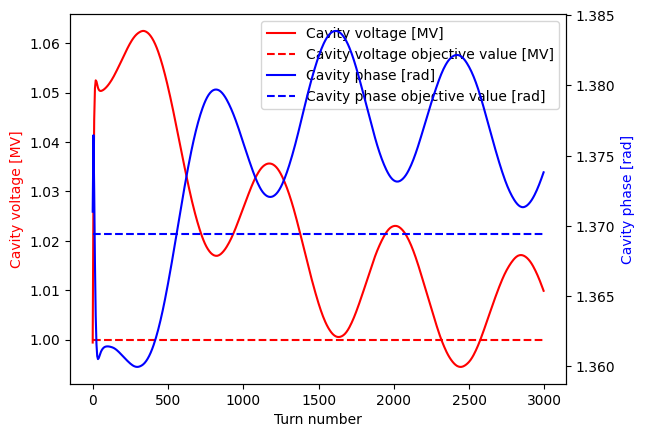
The CavityResonator setpoint (CavityResonator.Vc for the amplitude and CavityResonator.theta for the phase) can be shown along the data from tracking using the show_objective=True option of the plot_cavitydata function.

fig = plot_cavitydata("save.hdf5","MC", show_objective=True)

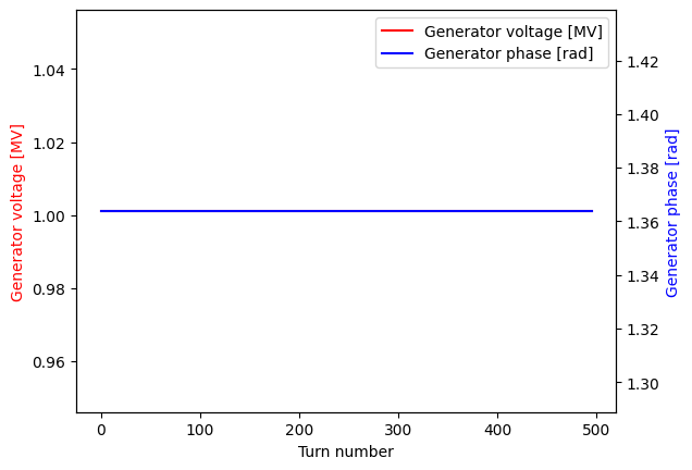
As there is no loop or feedback, the generator voltage/phase is constant:

fig = plot_cavitydata("save.hdf5","MC", phasor="generator")

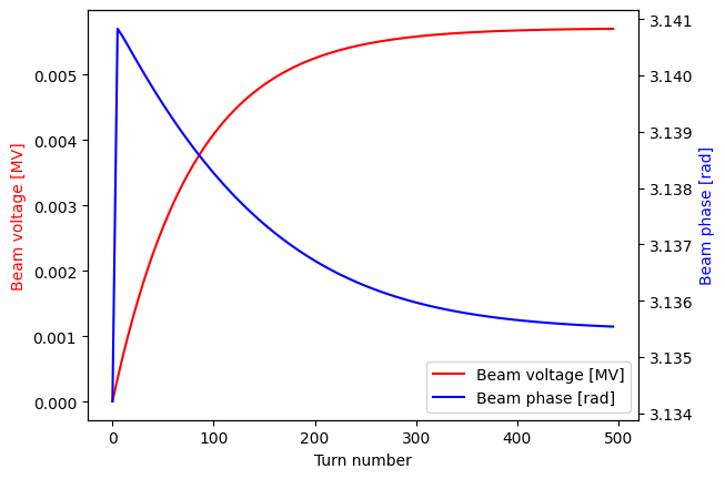
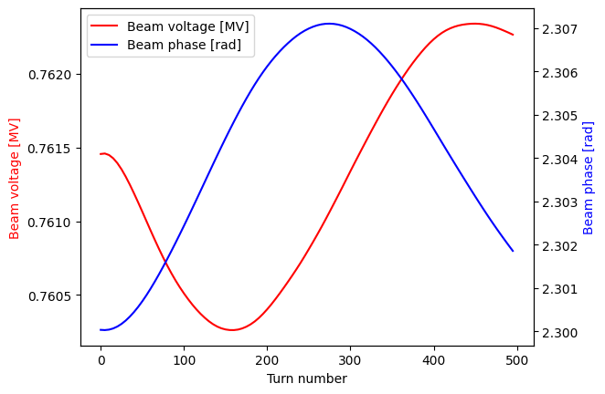
The beam voltage is nearly zero as the current is very low:

fig = plot_cavitydata("save.hdf5","MC", phasor="beam")

With beam

When including longtudinal motion and higher current (200 mA), it takes a bit longer for the cavity voltage and phase to converge to its design value as the beam loading needs to build up:

mybeam, MC, MCmon = restart(I0=0.2, tot_turns=3000)

for i in tqdm(range(3000)):
  long.track(mybeam)
  rad.track(mybeam)
  MC.track(mybeam)
  MCmon.track(mybeam, MC)
meanVc = np.mean(MC.cavity_phasor_record)
print(f"\n Residual error: amplitude {np.round((1-np.abs(meanVc)/MC.Vc)*100,3)} % & phase {np.round((1-np.angle(meanVc)/MC.theta)*100,3)} %")

100%|██████████| 3000/3000 [00:51<00:00, 58.79it/s]

 Residual error: amplitude -0.08 % & phase 0.048 %

fig = plot_cavitydata("save.hdf5","MC", show_objective=True)

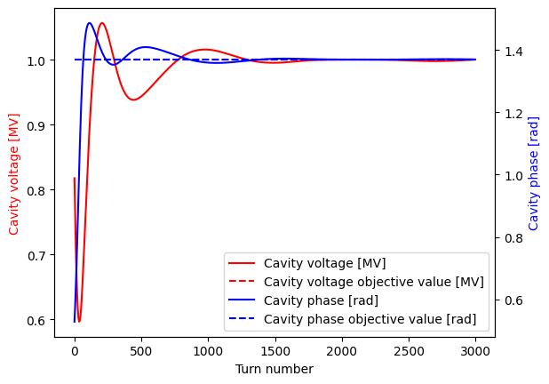
fig = plot_cavitydata("save.hdf5","MC", phasor="beam")

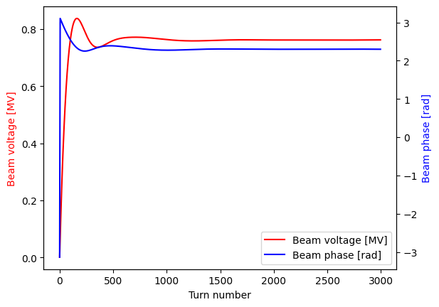
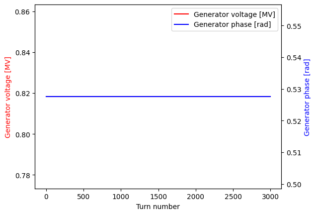
fig = plot_cavitydata("save.hdf5","MC", phasor="generator")

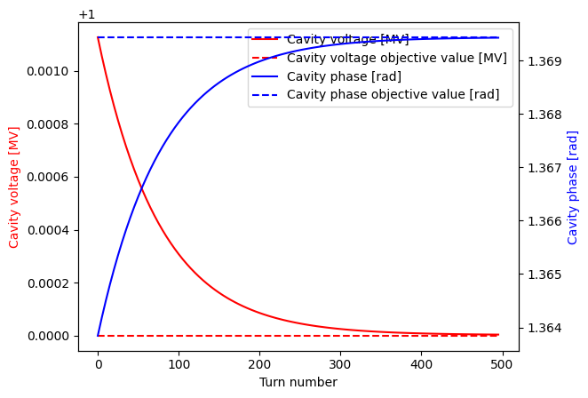
With beam and phasor initialization

To speed up the beam loading build-up, it is possible to use the CavityResonator.init_phasor method to initialize the CavityResonator.beam_phasor to its equilibrium value corresponding to a given beam distribution:

mybeam, MC, MCmon = restart(I0=0.2, tot_turns=500)

MC.init_phasor(mybeam)

for i in tqdm(range(500)):
  long.track(mybeam)
  rad.track(mybeam)
  MC.track(mybeam)
  MCmon.track(mybeam, MC)
meanVc = np.mean(MC.cavity_phasor_record)
print(f"\n Residual error: amplitude {np.round((1-np.abs(meanVc)/MC.Vc)*100,3)} % & phase {np.round((1-np.angle(meanVc)/MC.theta)*100,3)} %")

100%|██████████| 500/500 [00:09<00:00, 54.40it/s]

 Residual error: amplitude 0.1 % & phase -0.113 %

fig = plot_cavitydata("save.hdf5","MC", show_objective=True)

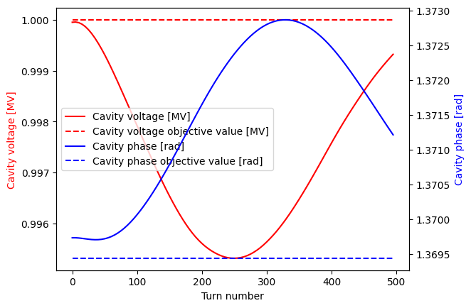
fig = plot_cavitydata("save.hdf5","MC", phasor="beam")

CavityResonator interface for loops and feedbacks

The different types of loop or feedback to be applied to CavityResonator objects are defined as separate classes, they must be initialised separately after the CavityResonator object.

The loop must then be added to the CavityResonator object using:

CavityResonator.feedback.append(loop)

The CavityResonator.feedback interface is just a list which contains all the different kinds of feedback applied to this CavityResonator object. Once a feedback has been added to this list, its track method will automatically be called when then CavityResonator.track method is called.

ProportionalLoop class

The ProportionalLoop is a simple proportional feedback loop to control a CavityResonator amplitude and phase. It takes as input:

• gain_A an amplitude (voltage) gain.

• gain_P a phase gain.

• delay the feedback delay in unit of turns.

The feedback setpoints are CavityResonator.Vc and CavityResonator.theta and the loop modifies the generator amplitude CavityResonator.Vg and phase CavityResonator.theta_g according to:

• Vg -= gain_A*(cavity_voltage - Vc)

• theta_g -= gain_P*(cavity_phase - theta)

The generator modification is applied after delay revolution periods.

from mbtrack2 import ProportionalLoop

Step without beam

The ProportionalLoop can be used to perform a step increase of the cavity voltage and phase.

mybeam, MC, MCmon = restart(I0=0.001, tot_turns=500)

MC.feedback

[]

MC.feedback is empty, let us define a ProportionalLoop object and adds it to MC:

PL = ProportionalLoop(ring, MC, gain_A=0.1, gain_P=0.1, delay=5)

MC.feedback.append(PL)

MC.feedback

[<mbtrack2.tracking.rf.ProportionalLoop at 0x7e8c5d7670a0>]

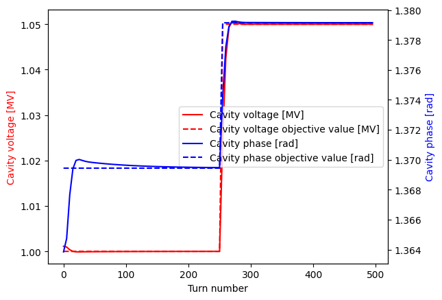
Here the objective voltage MC.Vc is increased to 1.05 MV at turn 250, the objective phase MC.theta is changed accordingly to keep energy balance:

for i in tqdm(range(500)):
  MC.track(mybeam)
  MCmon.track(mybeam, MC)
  if i == 250:
    MC.Vc = 1.05e6
    MC.theta = np.arccos(ring.U0/MC.Vc)
meanVc = np.mean(MC.cavity_phasor_record)
print(f"\n Residual error: amplitude {np.round((1-np.abs(meanVc)/MC.Vc)*100,3)} % & phase {np.round((1-np.angle(meanVc)/MC.theta)*100,3)} %")

100%|██████████| 500/500 [00:06<00:00, 74.47it/s]

 Residual error: amplitude 0.0 % & phase -0.0 %

fig = plot_cavitydata("save.hdf5","MC", show_objective=True)

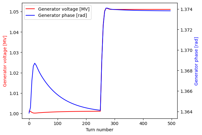
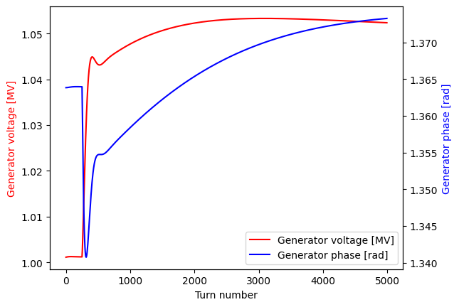
We can see that the generator voltage MC.Vg and phase MC.theta_g is changed by the ProportionalLoop during the tracking:

fig = plot_cavitydata("save.hdf5","MC", phasor="generator")

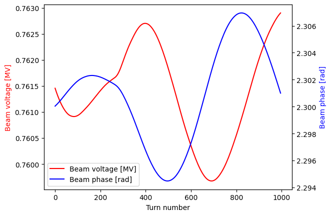
Step with beam

The same step with a 200 mA beam is shown bellow:

mybeam, MC, MCmon = restart(I0=0.2, tot_turns=1000)
MC.init_phasor(mybeam)

PL = ProportionalLoop(ring, MC, gain_A=0.1, gain_P=0.1, delay=5)
MC.feedback.append(PL)

for i in tqdm(range(1000)):
  long.track(mybeam)
  rad.track(mybeam)
  MC.track(mybeam)
  MCmon.track(mybeam, MC)
  if i == 250:
    MC.Vc = 1.05e6
    MC.theta = np.arccos(ring.U0/MC.Vc)
meanVc = np.mean(MC.cavity_phasor_record)
print(f"\n Residual error: amplitude {np.round((1-np.abs(meanVc)/MC.Vc)*100,3)} % & phase {np.round((1-np.angle(meanVc)/MC.theta)*100,3)} %")

100%|██████████| 1000/1000 [00:17<00:00, 56.14it/s]

 Residual error: amplitude -0.031 % & phase -0.061 %

fig = plot_cavitydata("save.hdf5","MC", show_objective=True)

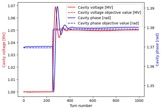
fig = plot_cavitydata("save.hdf5","MC", phasor="generator")

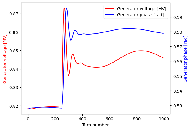
fig = plot_cavitydata("save.hdf5","MC", phasor="beam")

ProportionalIntegralLoop class

The ProportionalIntegralLoop is a more realistic Proportional Integral (PI) loop to control a CavityResonator amplitude and phase via generator current Ig to take into account the cavity response [1].

The basic idea of a PI controller is described here: https://en.wikipedia.org/wiki/PID_controller

The ProportionalIntegralLoop should be initialized only after generator parameters are set.

The ProportionalIntegralLoop important inputs are:

• gain a list of two float like [Pain, Igain], corresponding to the proportional gain Pain and integral gain Igain of the feedback.

• sample_num, the number of bunch over which the cavity amplitude and phase is computed (in unit of bucket number).

• every, the time interval between two cavity voltage monitoring and feedback in unit of bucket number. This corresponds to the update rate of the feedback.

• delay the loop delay in unit of bucket number.

The feedback setpoints are CavityResonator.Vc and CavityResonator.theta and the loop modifies the generator amplitude CavityResonator.Vg and phase CavityResonator.theta_g.

---

During the CavityResonator.track call, at each every RF bucket:

• The cavity_phasor is computed as the mean over sample_num buckets.

• The following calculation are done:

  • diff = (Vc*exp(1j*theta) - cavity_phasor) - FFconst where FFconst is the feedfoward constant.

  • I_record = I_record + diff/fRF where fRF is the RF frequency.

  • FB_val = Pain * diff + Igain * I_record

  • Ig = Vg2Ig(FB_val) + FFconst where Vg2Ig is a function to go from generator voltage to generator current.

• Ig is applied after delay RF buckets.

• Ig is then transformed back to generator voltage and modifies Vg and theta_g.

See [1] for the description on how to go from Ig to Vg and opposite.

---

Typical gain values:

• For normal conducting cavities (QL~1e4), a Pgain of ~1.0 and Igain of ~1e4(5) are usually used.

• For super conducting cavity (QL > 1e6), a Pgain of ~100 can be used.

In a “bad” parameter set, an unstable oscillation of the cavity voltage can be caused. So, a parameter scan of the gain should be made.

Some example parameters for KEK-PF:

FPGA-based LLRF controller, IQ sampling using 8 rf waves, output signal in 77-MHz, around 1us system delay

• E0=2.5GeV, C=187m, frf=500MHz

• QL=11800, fs0=23kHz

• ==> gain=[0.5,1e4], sample_num=8, every=7(13ns), delay=500(1us)

from mbtrack2 import ProportionalIntegralLoop

Step without beam

The same voltage step is applied using the ProportionalIntegralLoop without beam:

mybeam, MC, MCmon = restart(I0=0.001, tot_turns=5000)
MC.init_phasor(mybeam)

PIL = ProportionalIntegralLoop(ring, MC, gain=[1.5, 2e4], sample_num=5, every=5, delay=0)
MC.feedback.append(PIL)

for i in tqdm(range(5000)):
  MC.track(mybeam)
  MCmon.track(mybeam, MC)
  if i == 250:
    MC.Vc = 1.05e6
    MC.theta = np.arccos(ring.U0/MC.Vc)
meanVc = np.mean(MC.cavity_phasor_record)
print(f"\n Residual error: amplitude {np.round((1-np.abs(meanVc)/MC.Vc)*100,3)} % & phase {np.round((1-np.angle(meanVc)/MC.theta)*100,3)} %")

100%|██████████| 5000/5000 [01:15<00:00, 66.30it/s]

 Residual error: amplitude -0.126 % & phase 0.039 %

fig = plot_cavitydata("save.hdf5","MC", show_objective=True)

The current generator phasor Ig is changed by the ProportionalIntegralLoop during the tracking:

fig = plot_cavitydata("save.hdf5","MC", phasor="ig")

Which induces changes to the generator voltage and phase:

fig = plot_cavitydata("save.hdf5","MC", phasor="generator")

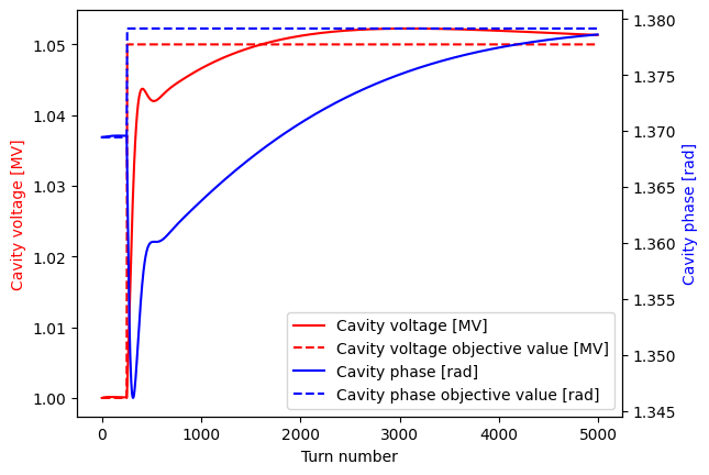
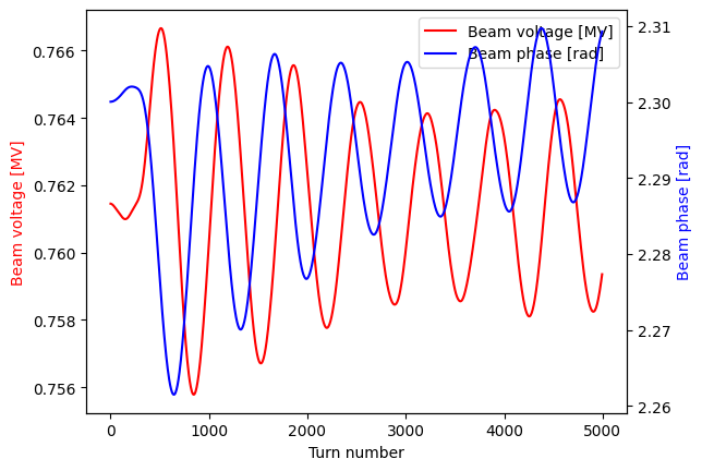
Step with beam

And now with a 200 mA beam:

mybeam, MC, MCmon = restart(I0=0.2, tot_turns=5000)
MC.init_phasor(mybeam)

PIL = ProportionalIntegralLoop(ring, MC, gain=[1.5, 2e4], sample_num=5, every=5, delay=0)
MC.feedback.append(PIL)

for i in tqdm(range(5000)):
  long.track(mybeam)
  rad.track(mybeam)
  MC.track(mybeam)
  MCmon.track(mybeam, MC)
  if i == 250:
    MC.Vc = 1.05e6
    MC.theta = np.arccos(ring.U0/MC.Vc)
meanVc = np.mean(MC.cavity_phasor_record)
print(f"\n Residual error: amplitude {np.round((1-np.abs(meanVc)/MC.Vc)*100,3)} % & phase {np.round((1-np.angle(meanVc)/MC.theta)*100,3)} %")

100%|██████████| 5000/5000 [01:28<00:00, 56.52it/s]

 Residual error: amplitude 0.283 % & phase 0.13 %

fig = plot_cavitydata("save.hdf5","MC", show_objective=True)

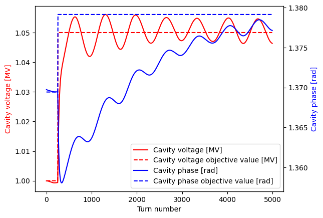
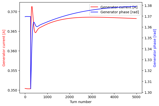
fig = plot_cavitydata("save.hdf5","MC", phasor="ig")

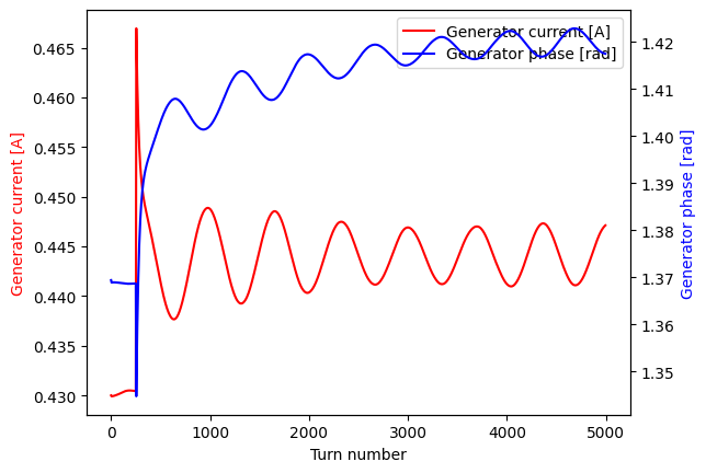
fig = plot_cavitydata("save.hdf5","MC", phasor="generator")

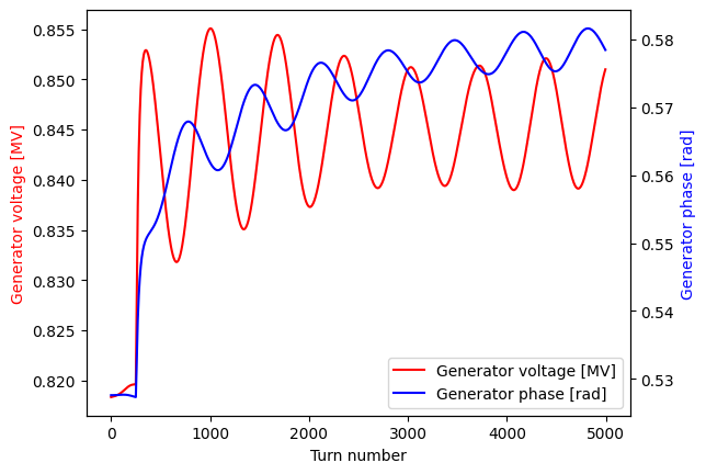
fig = plot_cavitydata("save.hdf5","MC", phasor="beam")

TunerLoop

The TunerLoop is used to control a CavityResonator tuning (CavityResonator.psi or CavityResonator.detune) in order to keep the phase between cavity and generator current constant.

The TunerLoop keeps the relation cavity_phase - theta_g + psi = offset constant using a proportional controller. The condition cavity_phase - theta_g + psi = 0 corresponds to the optimal tuning (minimum reflected power) of the CavityResonator.

The important inputs of TunerLoop are:

• gain, proportional gain of the tuner loop.

• avering_period, period during which the phase difference is monitored and averaged. Then the feedback correction is applied every avering_period turn. A value longer than one synchrotron period is recommended.

• offset, the tuning offset in [rad].

from mbtrack2 import TunerLoop

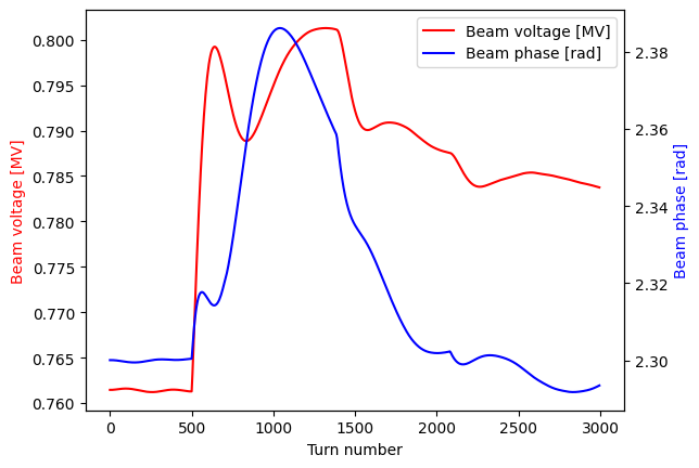
Current ramp-up

The TunerLoop can be used to keep the relation cavity_phase - theta_g + psi = offset constant during a current ramp-up from 200 mA to 210 mA:

mybeam, MC, MCmon = restart(I0=0.2, tot_turns=3000)
MC.init_phasor(mybeam)

nus = ring.synchrotron_tune(1.0e6) # synchrotron tune
Ts = 1/nus # synchrotron period in turns

Ts

693.5479215314126

TL = TunerLoop(ring, MC, gain=0.2, avering_period=Ts, offset=0)
MC.feedback.append(TL)

for i in tqdm(range(3000)):
  long.track(mybeam)
  rad.track(mybeam)
  MC.track(mybeam)
  MCmon.track(mybeam, MC)
  if i == 500:
    for i in range(ring.h):
      mybeam[i].current=mybeam[i].current*1.05 # 5 % current increase
meanVc = np.mean(MC.cavity_phasor_record)
print(f"\n Residual error: amplitude {np.round((1-np.abs(meanVc)/MC.Vc)*100,3)} % & phase {np.round((1-np.angle(meanVc)/MC.theta)*100,3)} %")

100%|██████████| 3000/3000 [01:18<00:00, 38.39it/s]

 Residual error: amplitude -1.699 % & phase -1.144 %

mybeam.current

0.21000000000000005

Because of the current increase, the beam loading voltage has increased:

fig = plot_cavitydata("save.hdf5","MC", show_objective=True)

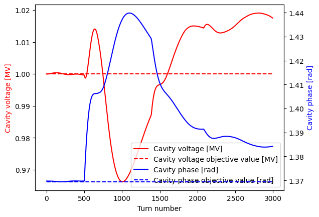
fig = plot_cavitydata("save.hdf5","MC", phasor="beam")

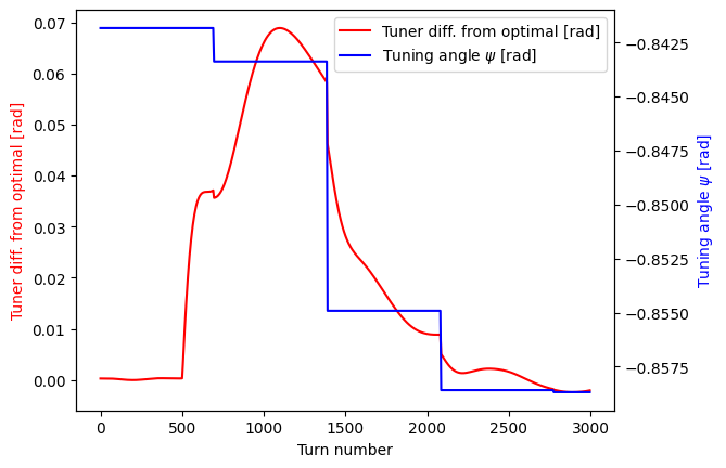
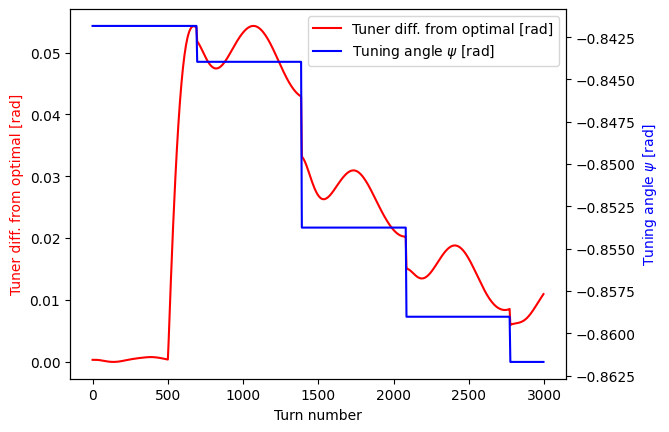
The cavity tuning angle CavityResonator.psi is controlled by the TunerLoop to keep the tuner difference constant:

fig = plot_cavitydata("save.hdf5","MC", plot_type="tuner_diff")

Current ramp-up with ProportionalIntegralLoop and TunerLoop

To keep both the cavity voltage and tuning constant during a current ramp-up, both ProportionalIntegralLoop and TunerLoop can be used at the same time:

mybeam, MC, MCmon = restart(I0=0.2, tot_turns=3000)
MC.init_phasor(mybeam)

PIL = ProportionalIntegralLoop(ring, MC, gain=[1.5, 2e4], sample_num=5, every=5, delay=0)
MC.feedback.append(PIL)

TL = TunerLoop(ring, MC, gain=0.2, avering_period=Ts, offset=0)
MC.feedback.append(TL)

MC.feedback

[<mbtrack2.tracking.rf.ProportionalIntegralLoop at 0x7e8c5d5ea470>,
 <mbtrack2.tracking.rf.TunerLoop at 0x7e8c5d5e9900>]

for i in tqdm(range(3000)):
  long.track(mybeam)
  rad.track(mybeam)
  MC.track(mybeam)
  MCmon.track(mybeam, MC)
  if i == 500:
    for i in range(ring.h):
      mybeam[i].current=mybeam[i].current*1.05 # 5 % current increase
meanVc = np.mean(MC.cavity_phasor_record)
print(f"\n Residual error: amplitude {np.round((1-np.abs(meanVc)/MC.Vc)*100,3)} % & phase {np.round((1-np.angle(meanVc)/MC.theta)*100,3)} %")

100%|██████████| 3000/3000 [01:17<00:00, 38.62it/s]

 Residual error: amplitude 0.73 % & phase 0.427 %

mybeam.current

0.21000000000000005

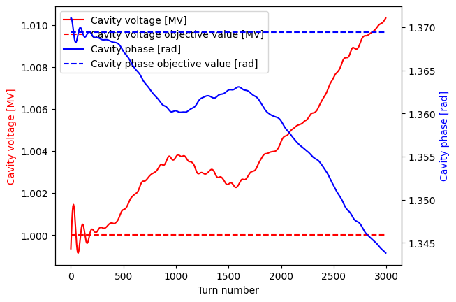
fig = plot_cavitydata("save.hdf5","MC", show_objective=True)

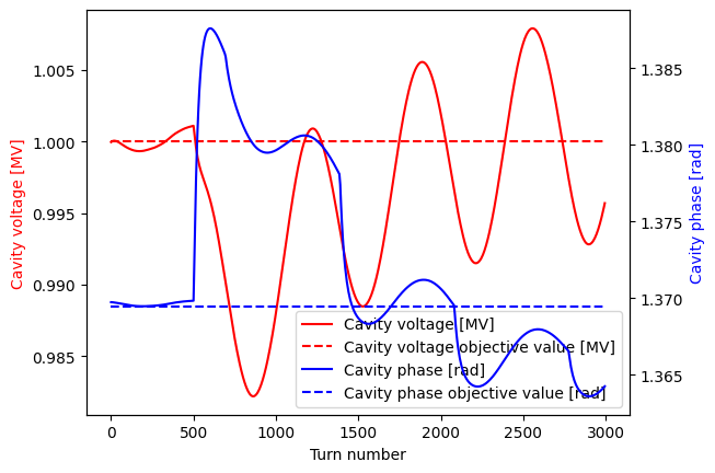
fig = plot_cavitydata("save.hdf5","MC", plot_type="tuner_diff")

DirectFeedback

The DirectFeedback is a direct RF feedback (DFB) [2,3] aiming to reduce the effective shunt impedance seen by the beam to fight against instabilities. It works by using a PI controller via generator current Ig to take into account the cavity response [1].

In fact, the DirectFeedback inherits from ProportionalIntegralLoop so all mandatory parameters from ProportionalIntegralLoop should be passed as kwargs when initializing a DirectFeedback object.

To avoid cavity-beam unmatching (large synchrotron oscilation of beam), the CavityResonator generator parameters should be set before initialization.

The DirectFeedback important inputs are:

• DFB_gain is the DFB gain.

• DFB_phase_shift is the DFB phase shift.

• gain,sample_num, every and delay for the ProportionalIntegralLoop must be specified.

• DFB_sample_num, DFB_every, DFB_delay are analog to their definitions in ProportionalIntegralLoop but the DirectFeedback. If not specified they take the same values as sample_num, every and delay.

---

The DFB induces a new generator voltage phasor component \(\tilde{V}_{g,DFB}\) which tends to reduce the effect of the beam loading, see [2,3] for more details.

During the CavityResonator.track call, at each DFB_every RF bucket:

• The cavity_phasor is computed as the mean over DFB_sample_num buckets.

• The following calculation are done:

  • Vg_DFB = DFB_gain * cavity_phasor * exp(1j*DFB_phase_shift).

  • Ig_DFB = Vg2Ig(Vg_DFB) where Vg2Ig is a function to go from generator voltage to generator current.

• Ig_DFB is applied after DFB_delay RF buckets.

• The total Ig is then transformed back to generator voltage and modifies Vg and theta_g.

See [1] for the description on how to go from Ig to Vg and opposite.

DC Robinson instability

The DC Robinson instability is a well known instability which leads to a loss of phase focusing if the beam loading voltage is too high compared to the generator voltage.

To illustrate this instability, we can track a 1 A beam and look at the results:

from mbtrack2 import BeamMonitor, plot_beamdata

I0 = 1.0
mybeam, MC, MCmon = restart(I0=I0, tot_turns=3000)
MC.init_phasor(mybeam)
beammon = BeamMonitor(ring.h, 10, 1, 300)

Check DC Robinson stability:

MC.is_DC_Robinson_stable(I0)

False

for i in tqdm(range(3000)):
  long.track(mybeam)
  rad.track(mybeam)
  MC.track(mybeam)
  MCmon.track(mybeam, MC)
  beammon.track(mybeam)
meanVc = np.mean(MC.cavity_phasor_record)
print(f"\n Residual error: amplitude {np.round((1-np.abs(meanVc)/MC.Vc)*100,3)} % & phase {np.round((1-np.angle(meanVc)/MC.theta)*100,3)} %")

100%|██████████| 3000/3000 [00:57<00:00, 52.02it/s]

 Residual error: amplitude 25.229 % & phase -48.969 %

The beam center of mass goes to infinity very fast in DC Robinson conditions:

fig = plot_beamdata("save.hdf5")

fig = plot_cavitydata("save.hdf5","MC", show_objective=True)

With DirectFeedback

With DirectFeedback, it is possible to reduce the effective shunt impedance Rs seen by the beam to recover stability in the same conditions as before (1 A beam):

from mbtrack2 import DirectFeedback

I0 = 1.0
mybeam, MC, MCmon = restart(I0=I0, tot_turns=3000)
MC.init_phasor(mybeam)
beammon = BeamMonitor(ring.h, 10, 1, 300)

DFB = DirectFeedback(ring=ring, cav_res=MC, gain=[1.5, 2e4], sample_num=5, every=5, delay=0, DFB_gain=0.1, DFB_phase_shift=0, DFB_sample_num=1, DFB_every=1)
MC.feedback.append(DFB)

MC.Rs*1e-6 # nominal shunt impedance in [Mohm]

20.0

DFB.DFB_Rs*1e-6 # effective shunt impedance in [Mohm]

19.61676229835558

With the effective shunt impedance, the 1 A beam should be stable:

MC.Rs = DFB.DFB_Rs
print(MC.is_DC_Robinson_stable(I0))
MC.Rs = 20e6

True

for i in tqdm(range(3000)):
  long.track(mybeam)
  rad.track(mybeam)
  MC.track(mybeam)
  MCmon.track(mybeam, MC)
  beammon.track(mybeam)
meanVc = np.mean(MC.cavity_phasor_record)
print(f"\n Residual error: amplitude {np.round((1-np.abs(meanVc)/MC.Vc)*100,3)} % & phase {np.round((1-np.angle(meanVc)/MC.theta)*100,3)} %")

100%|██████████| 3000/3000 [00:59<00:00, 50.71it/s]

 Residual error: amplitude -0.911 % & phase -0.34 %

fig = plot_beamdata("save.hdf5")

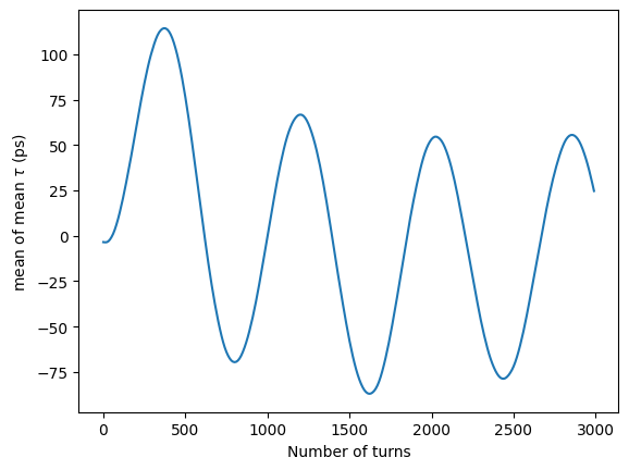
fig = plot_cavitydata("save.hdf5","MC", show_objective=True)