![]()
Introduction
This notebook introduces how set-up a tracking simulation including single bunch and multi-bunch collective effects in mbtrack2.
The following classes are used to prepare a simulation with collective effects or more generally to make computations with impedance and wake functions:
The
Impedanceclass is used to store impedance data.The
WakeFunctionclass is used to store wake function data.The
WakeFieldclass is used to represent a single physical element which produces different types of wakes, represented byImpedanceorWakeFunctionobjects.The
ImpedanceModelclass is used to sum differentWakeFieldelements taking into account betatron function weighting.
These other classes are used in tracking to deal with single bunch and multi-bunch collective effects:
The
WakePotentialclass deals with the single bunch effects, it can be used in tracking to model:Longituinal (monopole) wake potential
Transverse monopole wake potential
Transverse dipole wake potential
Transverse quadrupolar wake potential
The
WakePotentialMonitorclass is used to monitorWakePotentialobjects and save its differents attributes (wake potentials, bunch profile, dipole moments, …) during tracking.The
LongRangeResistiveWallclass is used to deal with multi-bunch and multi-turn (longitudinal and tranverse) wakes from resistive wall using the algorithm defined in [1].
References
[1] Skripka, Galina, et al. “Simultaneous computation of intrabunch and interbunch collective beam motions in storage rings.” NIM.A (2016).
[2] Zotter, Bruno W., and Semyon A. Kheifets. Impedances and wakes in high-energy particle accelerators. World Scientific, 1998.
[3] Gamelin, Alexis. “Collective effects in a transient micro-bunching regime and ion cloud mitigation in ThomX.” (2018).
Initialization
mbtrack2 set-up
pip install mbtrack2
Define a Synchrotron object
import numpy as np
from mbtrack2 import Synchrotron, Electron, Optics
h = 20 # Harmonic number of the accelerator.
L = 100 # Ring circumference in [m].
E0 = 1.5e9 # Nominal (total) energy of the ring in [eV].
particle = Electron() # Particle considered.
ac = 1e-3 # Momentum compaction factor.
U0 = 200e3 # Energy loss per turn in [eV].
tau = np.array([1e-3, 1e-3, 2e-3]) # Horizontal, vertical and longitudinal damping times in [s].
tune = np.array([12.2, 15.3]) # Horizontal and vertical tunes.
emit = np.array([10e-9, 10e-12]) # Horizontal and vertical equilibrium emittance in [m.rad].
sigma_0 = 15e-12 # Natural bunch length in [s].
sigma_delta = 1e-3 # Equilibrium energy spread.
chro = [2.0, 3.0] # Horizontal and vertical (non-normalized) chromaticities.
local_beta = np.array([3, 2]) # Beta function at the tracking location.
local_alpha = np.array([0, 0]) # Alpha function at the tracking location.
local_dispersion = np.array([0, 0, 0, 0]) # Dispersion function and its derivative at the tracking location.
optics = Optics(local_beta=local_beta, local_alpha=local_alpha,
                  local_dispersion=local_dispersion)
ring = Synchrotron(h=h, optics=optics, particle=particle, L=L, E0=E0, ac=ac,
                   U0=U0, tau=tau, emit=emit, tune=tune,
                   sigma_delta=sigma_delta, sigma_0=sigma_0, chro=chro)
Define Bunch and Beam objects
from mbtrack2 import Beam, Bunch
mybunch = Bunch(ring,  mp_number=1e5, current=1e-3)
mybunch.init_gaussian()
filling_pattern = np.ones(ring.h)*0.025
mybeam = Beam(ring)
mybeam.init_beam(filling_pattern, mp_per_bunch=1e3)
Working with impedances
Conventions
The wake function and impedance conventions for mbtrack2 follow the ones from the book “Impedances and wakes in high-energy particle accelerators” from Zotter and Kheifets [2].
Also keep in mind that in mbtrack2, the head of the bunch is given for \(\tau < 0\) and thus the tail is for \(\tau > 0\).
Wake functions
The longitudinal wake function \(W_{\parallel}\) is defined as: $\(W_{\parallel} (z) = - \frac{1}{q} \int_{-\infty}^{+\infty} E_{\parallel} (z) dz\)$
Using this convention, a positive wake function corresponds to energy loss.
The transverse dipolar wake function \(W_{\perp}^{D}\) is defined as: $\(W_{\perp}^{D} (z) = \frac{1}{q \xi} \int_{-\infty}^{+\infty} [ E_{\perp} (z) + v \times B (z) ] dz\)\( Where \)\xi$ is the transverse displacement of the source particle.
So using this convention, for a positive \(\xi\), a positive transverse dipolar wake function corresponds to defocusing i.e. a positive angular kick felt by the test particle.
Impedances
The longitudinal impedance \(Z_{\parallel}\) is defined as: $\(Z_{\parallel} (\omega) = \frac{-v}{q} \int_{-\infty}^{+\infty} E_{\parallel} (z) e^{\frac{j \omega z}{v}} \frac{dz}{v}\)$
The transverse dipolar impedance \(Z_{\perp}^{D}\) is defined as: $\(Z_{\perp}^{D} (\omega) = \frac{-jv}{q\xi} \int_{-\infty}^{+\infty} [ E_{\perp} (z) + v \times B (z) ] e^{\frac{j \omega z}{v}} \frac{dz}{v}\)$
Relations between impedances and wake functions
If \(v=c\), impedances and wake functions are simply related thourgh Fourier transforms. For the longtudinal impedance and wake function:
For the transverse dipolar impedance and wake function:
Relations with other ressources
How the mbtrack2 convention relates with other popular ressources or codes:
A. Chao “Physics of Collective Beam Instabilities in High Energy Accelerators” \(⟶\) Complex conjugate for both longitudinal and transverse impedance.
CST Studio \(⟶\) Same convention (for positive wake_shift in wake integration info).
ImpedanceWake2D \(⟶\) Same convention.
Impedance and WakeFunction classes
The Impedance class is used to store and make computation on impedance data while the WakeFunction one does the same for wakefunction data.
from mbtrack2 import Impedance, WakeFunction
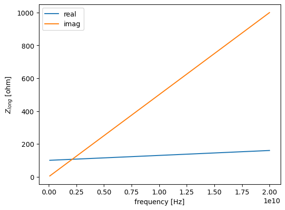
An Impedance object can be simply initialized by inputing the frequency points, impedance values and the impedance type:
variable = np.linspace(0.1e9, 20e9, 1000) # frequency points in [Hz]
function = 100 + variable*(3e-9 + 5e-8j) # impedance values in [Ohm]
component_type = "long" # type of the impedance
imp = Impedance(variable, function, component_type)
The impedance data in then stored in a pandas DataFrame accessible using:
imp.data
| real | imag | |
|---|---|---|
| frequency [Hz] | ||
| 1.000000e+08 | 100.300000 | 5.000000 |
| 1.199199e+08 | 100.359760 | 5.995996 |
| 1.398398e+08 | 100.419520 | 6.991992 |
| 1.597598e+08 | 100.479279 | 7.987988 |
| 1.796797e+08 | 100.539039 | 8.983984 |
| ... | ... | ... |
| 1.992032e+10 | 159.760961 | 996.016016 |
| 1.994024e+10 | 159.820721 | 997.012012 |
| 1.996016e+10 | 159.880480 | 998.008008 |
| 1.998008e+10 | 159.940240 | 999.004004 |
| 2.000000e+10 | 160.000000 | 1000.000000 |
1000 rows × 2 columns
The usual methods available on DataFrame are then usable, and a shorcut to plot the data is available:
ax = imp.plot()
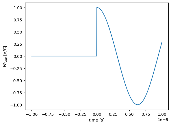
The WakeFunction class works in a similar way:
variable = np.linspace(-1e-9, 1e-9, 1000) # time points in [s]
function = np.cos(variable*5e9) # wake function values in [V/C]
ind = variable < 0
function[ind] = 0
component_type = "long" # type of the wake function
wake = WakeFunction(variable, function, component_type)
ax = wake.plot()
The list of possible types for Impedance and WakeFunction objects is:
"long"for (monopoloar) longitudinal"xcst"for monopolar horizontal"ycst"for monopolar vertical"xdip"for dipolar horizontal"ydip"for dipolar vertical"xquad"for quadripolar horizontal"yquad"for quadripolar vertical
The type of the Impedance or WakeFunction can be checked using:
wake.component_type
'long'
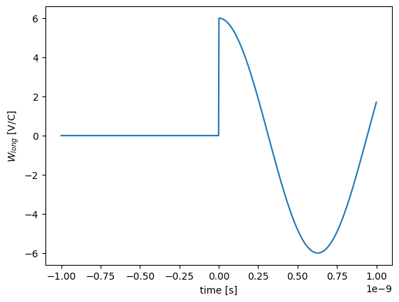
Linear algebra is possible on both Impedance and WakeFunction objects of the same type:
new_wake = wake*5 + wake
ax = new_wake.plot()
Both Impedance and WakeFunction have a function-like behaviour and can be called at given points to get an interpolation of the data at theses points:
freq_points = [1e9, 5e9, 10e9] # in [Hz]
imp(freq_points) # interpolated data in [Ohm]
array([103. +50.j, 115.+250.j, 130.+500.j])
The loss factor (or kick factor) can be computed for an Impedance assuming a Gaussian bunch using:
sigma = 15e-12 # RMS bunch length in [s]
imp.loss_factor(sigma) # in [V/C] or kick factor in [V/C/m] depanding on the impedance type.
np.float64(2174220483620.3323)
WakeField class
The WakeField class is based on a collection of Impedance and WakeFunction objects of different types. It usually corresponds to a single physical element which produces different types of wakes.
from mbtrack2 import WakeField
It can be initialized from a list of Impedance and WakeFunction objects of different types:
wakefield = WakeField([wake, imp], name="my wake")
The different components can then be accessed through the Z + component_type attribute for Impedance objects and through the W + component_type attribute for WakeFunction objects:
ax = wakefield.Wlong.plot()
The list of components can be accessed and manipulated using the class methods:
wakefield.components # show components list
array(['Wlong', 'Zlong'], dtype='<U5')
wakefield.drop("Zlong") # remove component from WakeField
wakefield.append_to_model(WakeFunction(variable, function, "xdip")) # add component to WakeField
wakefield.components # show components list
array(['Wlong', 'Wxdip'], dtype='<U5')
The Wakefield representation also shows the Wakefield name field and its components:
wakefield
WakeField my wake with components:
 [np.str_('Wlong'), np.str_('Wxdip')]
The WakeField class provide two static methods to add WakeField objects togather taking into account betatron function weighting:
WakeField.add_wakefields(wake1, beta1, wake2, beta2)WakeField.add_several_wakefields(wakefields, beta)
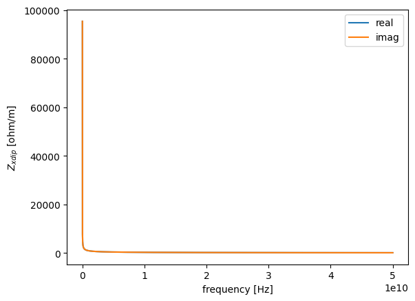
Many classes in mbtrack2 inherit from the WakeField class, usually to provide an implementation of the most commonly used formulas. For example, the CircularResistiveWall class provide a resistive wall WakeField element for a circular beam pipe:
from mbtrack2 import CircularResistiveWall

time = np.linspace(0, 200e-12, 10000) # Time points where the wake function will be evaluated in [s].
frequency = np.linspace(0.1e6, 50e9, 10000) # Frequency points where the impedance will be evaluated in [Hz].
length = 1 # Beam pipe length in [m].
rho = 1e-6 # Resistivity in [ohm.m].
radius = 10e-3 # Beam pipe radius in [m].
exact = True # If False, approxmiated formulas are used for the wake function computations.

rw = CircularResistiveWall(time, frequency, length, rho, radius, exact)
ax = rw.Zxdip.plot()
ax = rw.Wxdip.plot()
Importing from external sources
In many cases, it is much more pratical (or needed) to import the impedance or wake function data from other sources. A few functions are provided to import data from other codes:
read_CSTto read CST text file format into anImpedanceorWakeFunctionobject.read_IW2Dandread_IW2D_folderto read IW2D files into anImpedanceobject, aWakeFunctionobject or directly into aWakeFieldobject.read_ABCIto read ABCI output .pot files into aWakeFieldobject.read_ECHO2Dto read ECHO2D text file format (after matlab post-processing) into aWakeFunctionobject.
The Impedance class also has a to_wakefunction method and theWakeFunction class has both a to_impedance and a deconvolution method. They can be used to go from Impedance to WakeFunction and vice versa using FFT.
The deconvolution method can be used to compute a “pseudo wake function” from wake potential data (usually obtained from EM simulation). The computation uses a simple deconvolution method [3] and, of course, the frequency content (and thus the validity) of the ouput impedance or wake function data depends on the input wake potential.
ImpedanceModel class
The ImpedanceModel class is used to sum different WakeField elements taking into account betatron function weighting.
from mbtrack2 import ImpedanceModel
model = ImpedanceModel(ring)
The ImpedanceModel class uses the lattice information stored in ring.optics to access the betatron functions along the ring. So the full betatron functions must be available in ring.optics to be able to do the betatron weigthing of the transverse impedance and wake functions correctly.
ring.optics.use_local_values
True
The last command shows that for the ring Synchrotron object loaded here it is not the case and only local values are available. To make it available, the data must be added using the load_from_AT method from the Optics class to load at Accelerator Toolbox lattice file.
The transverse components of the summed WakeField computed by the model is normalized to the local beta function used for tracking:
ring.optics.local_beta
array([3, 2])
In this example, we will just assume that the beta function is constant along the ring:
ring.optics.beta([0, 25, 50]) # H/V beta function at s = 0, 25, 50 m in [m]
array([[3, 3, 3],
       [2, 2, 2]])
Then the different contributors to the ImpedanceModel must be added. This can be done in one of two ways, depending on the type of WakeField being added:
If the
WakeFieldis of the lumped type, usually corresponding to a geometric component at a given position in the lattice, then theaddmethod is used.If the
WakeFieldis of the distributed type, usually corresponding to a resistive wall component with an effective radius that already takes beta weighting into account, then theadd_globalmethod is used.
In the latter case, the WakeField element is added only after the summation of all the lumped type elements added with the add method.
from mbtrack2 import Resonator
For this example, we will sum different Resonator elements:
time = np.linspace(0,200e-12, int(1e5))
frequency = np.linspace(0.01e9, 50e9, int(1e5))
res1 = Resonator(time, frequency, Rs=10e3, fr=10e9, Q=60, plane="long")
res2 = Resonator(time, frequency, Rs=30e3, fr=5e9, Q=40, plane="long")
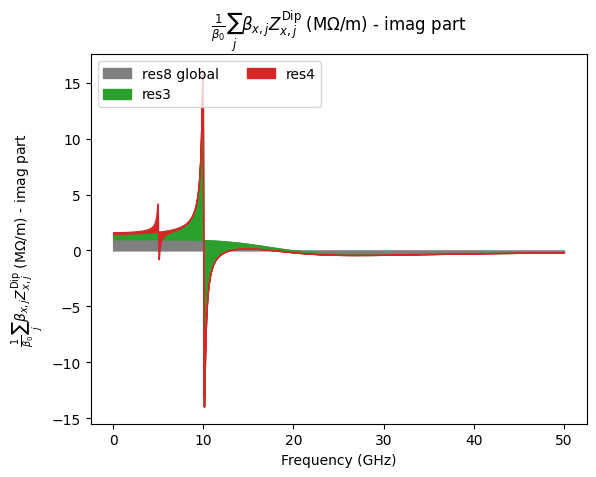
res3 = Resonator(time, frequency, Rs=10e6, fr=10e9, Q=60, plane="x")
res4 = Resonator(time, frequency, Rs=5e6, fr=5e9, Q=40, plane="x")
res5 = Resonator(time, frequency, Rs=10e6, fr=10e9, Q=60, plane="y")
res6 = Resonator(time, frequency, Rs=5e6, fr=5e9, Q=40, plane="y")
res7 = Resonator(time, frequency, Rs=5000, fr=20e9, Q=1, plane="long")
res8 = Resonator(time, frequency, Rs=1e6, fr=20e9, Q=1, plane="x")
res9 = Resonator(time, frequency, Rs=1e6, fr=20e9, Q=1, plane="y")
Then we can add them to the ImpedanceModelobject by giving the positions the elements along the lattice and a name:
model.add(wakefield=res1, positions=[22, 44], name="res1")
model.add(wakefield=res2, positions=[33], name="res2")
model.add(wakefield=res3, positions=[12, 15, 36], name="res3")
model.add(wakefield=res4, positions=[52], name="res4")
model.add(wakefield=res5, positions=[4, 6, 20], name="res5")
model.add(wakefield=res6, positions=[44, 53], name="res6")
model.add_global(wakefield=res7, name="res7 global")
model.add_global(wakefield=res8, name="res8 global")
model.add_global(wakefield=res9, name="res9 global")
Finaly, the compute_sum method must be called when all the components have been added:
model.compute_sum()
The result is a sum WakeField object which can be used for tracking or for plotting purpose:
model.sum
WakeField sum with components:
 [np.str_('Wlong'), np.str_('Wxdip'), np.str_('Wydip'), np.str_('Zlong'), np.str_('Zxdip'), np.str_('Zydip')]
model.sum.Wxdip.plot()
<Axes: xlabel='time [s]', ylabel='$W_{xdip}$ [V/C/m]'>
The contribution of each component can be analysed using the plot_area method:
fig = model.plot_area(Z_type="Zlong", component="real")
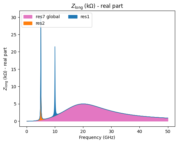
fig = model.plot_area(Z_type="Zxdip", component="imag")
Tracking with collective effects
WakePotential class
The WakePotential class is used to model the single bunch collective effects, it computes wake potentials in time domain from uniformly sampled wake functions by performing a convolution with a bunch charge profile.
Two different time bases are used. The first one is controled by the n_bin parameter and is used to compute the bunch profile. Then the bunch profile is interpolated on the wake function time base which is used to perform the convolution to get the wake potential.
As the computation is based on the input wake function, special care should be given on the choice of the time array. It should be long enough to cover twice the longest expected bunch length in the simulation and dense enough to correctly reproduce the wake function variation.
from mbtrack2 import WakePotential
wp = WakePotential(ring, wakefield=rw, n_bin=60)
The WakeField element given as input parameter to the WakePotential object determines which wake potential will be computed by the class.
For example, for the previously defined wakefield from the CircularResistiveWall class:
rw.wake_components
array(['Wlong', 'Wxdip', 'Wydip'], dtype='<U5')
The WakePotential object will compute and apply on the bunch the longitudinal, dipolar horizontal and dipolar vertical wake potentials using the track method:
wp.track(mybunch)
The last computed wake potential is stored in the class and can be plotted:
fig = wp.plot_last_wake("Wlong")
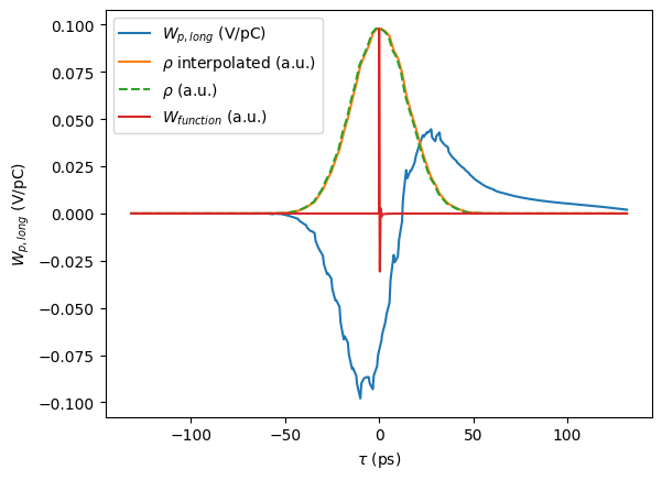
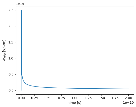
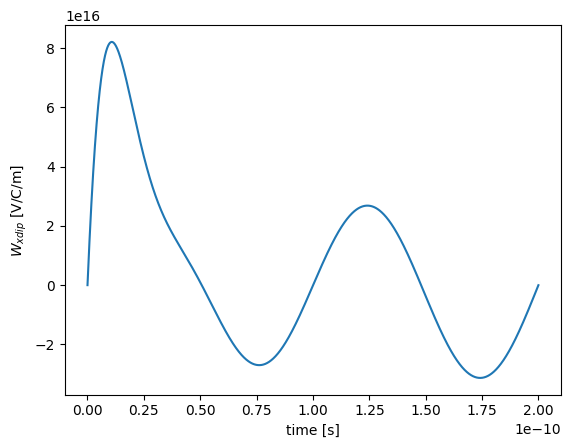
The dipole moment used to compute dipolar wake potential is also stored:
fig = wp.plot_last_wake("Wxdip", plot_dipole=True)
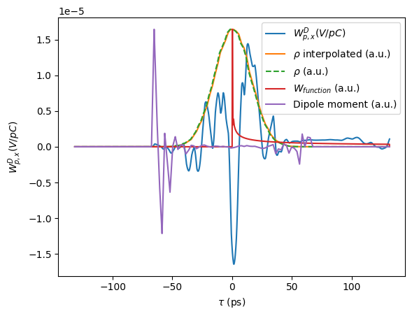
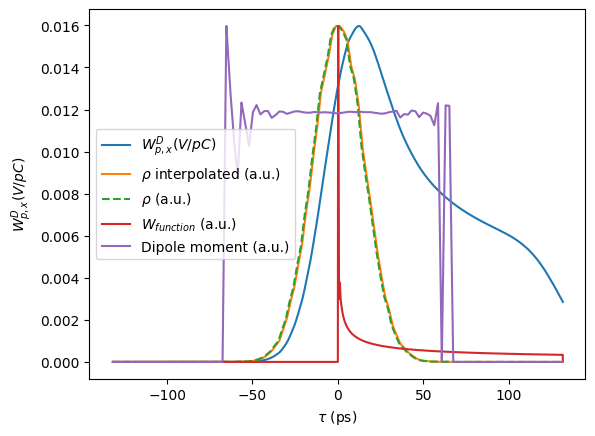
To be able to see the dipolar wake potential correct shape, the bunch need to be offsetted:
mybunch["x"] += 1e-3
mybunch["y"] += 1e-3
wp.track(mybunch)
fig = wp.plot_last_wake("Wxdip", plot_dipole=True)
It is possible to get a correctness estimate of the computed wake potentials using the reference_loss method.
It compares the loss factor (and kick factors) computed in time domain and in frequency domain:
The time domain (TD) value is computed using the wake potentials and bunch profile stored in the
WakePotentialobject (so from the lasttrackcall).The frequency domain (FD) value is computed assuming a Gaussian distribution and uses the impedance data stored in the
WakeFieldobject.
Both values should match assuming that the tracking bunch has a Gaussian distribution.
wp.reference_loss(mybunch)
| TD factor | FD factor | Relative error [%] | |
|---|---|---|---|
| Wlong [V/C] | 4.222085e+10 | 4.228940e+10 | -0.162098 |
| Wxdip [V/C/m] | 1.124837e+13 | 1.154082e+13 | -2.534103 |
| Wydip [V/C/m] | 1.124817e+13 | 1.154082e+13 | -2.535802 |
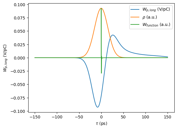
The input wake function can also be checked by computing the wake potential from a perfect Gaussian distribution:
fig = wp.plot_gaussian_wake(sigma=ring.sigma_0, wake_type="Wlong")
The track method of the WakePotential can also be used on Beam objects, each Bunch will compute and apply its own wake potential.
WakePotentialMonitor class
The WakePotentialMonitor class is used to monitor WakePotential objects and save its differents attributes (wake potentials, bunch profile, dipole moments, …) during tracking.
from mbtrack2 import WakePotentialMonitor
It is defined in the same way as other Monitor class objects, the bunch_number parameter is only used if a Beam object is tracked instead of a Bunch.
wp_mon = WakePotentialMonitor(bunch_number=0, wake_types=["Wlong","Wxdip","Wydip"], n_bin=60, save_every=1, buffer_size=10, total_size=100, file_name="save", mpi_mode=False)
The WakePotentialMonitor track method takes both the Bunch (or Beam) as first parameter and the WakePotential as second parameter.
Now let us set up a small tracking example with both WakePotential and WakePotentialMonitor objects:
from mbtrack2.tracking import LongitudinalMap, RFCavity, SynchrotronRadiation, TransverseMap
LongMap = LongitudinalMap(ring)
RF = RFCavity(ring, m=1, Vc=1e6, theta=np.arccos(ring.U0/1e6))
SR = SynchrotronRadiation(ring)
TransMap = TransverseMap(ring)
turns = 100
for i in range(turns):
  LongMap.track(mybunch)
  SR.track(mybunch)
  TransMap.track(mybunch)
  RF.track(mybunch)

  # collective effects part
  wp.track(mybunch)
  wp_mon.track(mybunch, wp)
The saved data can be accessed directly in the "save.hdf5" file or plotted directly using the plot_wakedata function:
from mbtrack2 import plot_wakedata
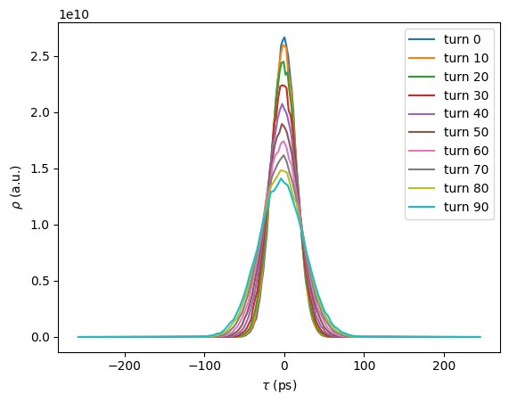
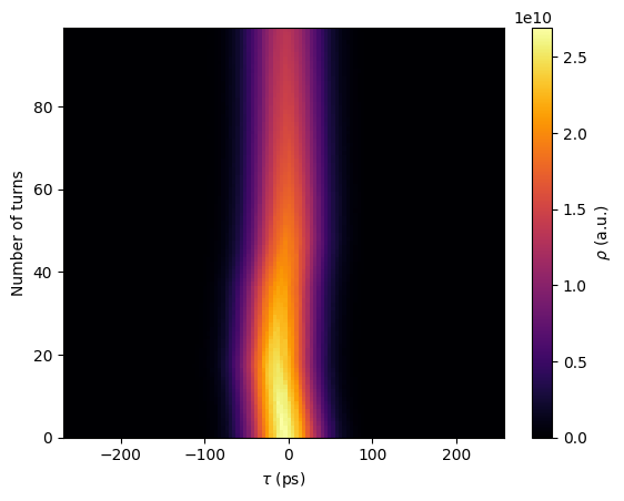
Here showing the longitudinal wake potential and bunch profile at different turns:
fig = plot_wakedata(filename="save.hdf5",bunch_number=0, wake_type="Wlong", start=0,
                     stop=None, step=10, streak_plot=False,
                     bunch_profile=False, dipole=False)
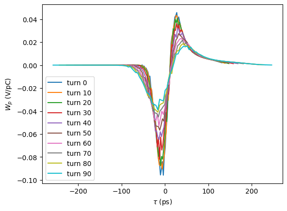
fig = plot_wakedata(filename="save.hdf5",bunch_number=0, wake_type="Wlong", start=0,
                     stop=None, step=10,streak_plot=False,
                     bunch_profile=True, dipole=False)
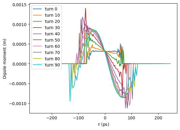
And the horizontal dipolar wake potential and dipole moment:
fig = plot_wakedata(filename="save.hdf5",bunch_number=0, wake_type="Wxdip", start=0,
                     stop=None, step=10, streak_plot=False,
                     bunch_profile=False, dipole=False)
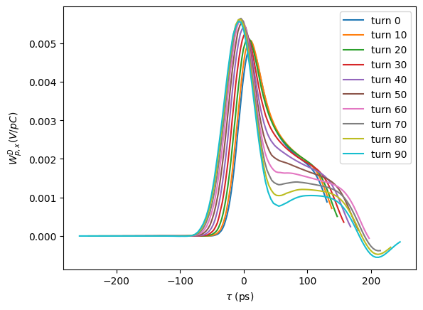
fig = plot_wakedata(filename="save.hdf5",bunch_number=0, wake_type="Wxdip", start=0,
                     stop=None, step=10, streak_plot=False,
                     bunch_profile=False, dipole=True)
The same data can also be plotted in “streak_plot” mode:
fig = plot_wakedata(filename="save.hdf5",bunch_number=0, wake_type="Wlong", start=0,
                     stop=None, step=None, streak_plot=True,
                     bunch_profile=False, dipole=False)
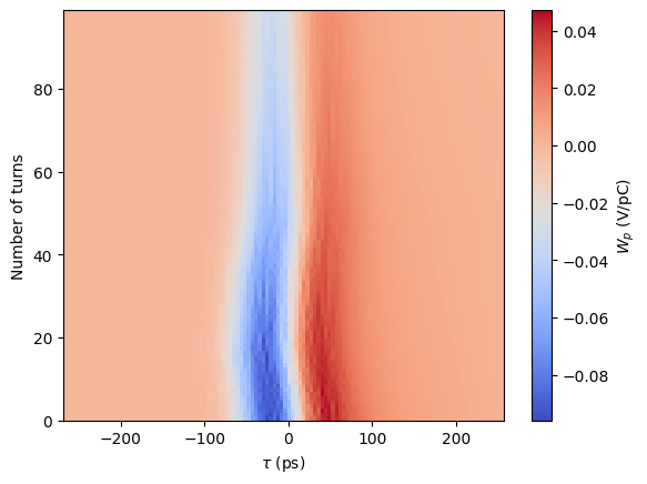
fig = plot_wakedata(filename="save.hdf5",bunch_number=0, wake_type="Wlong", start=0,
                     stop=None, step=None, streak_plot=True,
                     bunch_profile=True, dipole=False)
LongRangeResistiveWall class
The LongRangeResistiveWall class is used to deal with multi-bunch and multi-turn wakes from resistive wall using the algorithm defined in [1].
The main approximations done in this class:
Bunches are treated as point charge.
Assymptotic expression for the resistive wall wake functions are used.
Multi-turn wakes are limited to
ntturns.
Self-bunch interaction is not included in this class and should be dealed with the WakePotential class!
from mbtrack2 import LongRangeResistiveWall
length = 1 # Length of the resistive pipe to consider in [m].
rho = 1e-6 # Effective resistivity to consider in [ohm.m] as in [1].
radius = 10e-3 # Beam pipe radius to consider in [m].
types=["Wlong","Wxdip","Wydip"] # Wake types to consider.
nt=50 # Number of turns to consider for the long range wakes.
x3=None # Horizontal effective radius of the 3rd power in [m], as Eq.27 in [1]. The default is radius.
y3=None # Vertical effective radius of the 3rd power in [m], as Eq.27 in [1]. The default is radius.
The effective resistivity and radius, taking into account the betatron function averaging, as defined in [1] can be computed using the PhysicalModel class.
lrrw = LongRangeResistiveWall(ring=ring, beam=mybeam, length=length, rho=rho, radius=radius, types=types, nt=nt, x3=x3, y3=y3)
The LongRangeResistiveWall class can only be used with Beam objects and not with Bunch objects.
turns = 100
for i in range(turns):
  LongMap.track(mybeam)
  SR.track(mybeam)
  TransMap.track(mybeam)
  RF.track(mybeam)

  # collective effects part
  wp.track(mybeam) # single bunch wake
  lrrw.track(mybeam) # multi-bunch and multi-turn wake
/home/gamelina/Python_dev/mbtrack2_dir/mbtrack2/mbtrack2/tracking/wakepotential.py:963: RuntimeWarning: overflow encountered in scalar multiply
  np.sqrt(self.Z0 * self.rho / (c * pi * t**3)) * self.length) * -1
To model correctly the physics of the resistive wall, both the WakePotential (taking into account the resisitive wall wake function and possibly the broad band impedance) and the LongRangeResistiveWall are needed.