Coherent Synchrotron Radiation (CSR) Wakefields

This notebook introduces the FreeSpaceCSR and ParallelPlatesCSR classes from mbtrack2.impedance.csr, which model the coherent synchrotron radiation (CSR) wakefield.

CSR arises when a relativistic electron bunch travels along a curved trajectory (e.g. in a dipole magnet). The electrons radiate coherently at wavelengths comparable to or shorter than the bunch length, and the radiation field acts back on the bunch as a collective, self-induced force. CSR is an important effect in storage rings operating at short bunch lengths or high current, and is a key driver of microwave instabilities.

Two models are provided:

• FreeSpaceCSR: free-space steady-state model (no shielding).

• ParallelPlatesCSR: steady-state model with shielding by perfectly conducting parallel plates (vacuum chamber).

Both classes inherit from WakeField and provide an Impedance and a WakeFunction component.

References

[1] Faltens, A., & Laslett, L. J. (1973). Longitudinal coupling impedance of a stationary electron ring in a cylindrical geometry. Part. Accel., 4, 151–157.

[2] Agoh, T. and K. Yokoya. “Calculation of coherent synchrotron radiation using mesh.” Phys. Rev. ST Accel. Beams 7 (2004): 054403.

[3] E. L. Saldin, E. A. Schneidmiller, and M. V. Yurkov, “On the coherent radiation of an electron bunch moving in an arc of a circle”, Nucl. Instrum. Methods Phys. Res. A 398, 373 (1997).

[4] J. B. Murphy, S. Krinsky, and R. L. Gluckstern, “Longitudinal wakefield for an electron moving on a circular orbit”, Part. Accel. 57, 9 (1997).

Initialization

import numpy as np
import matplotlib.pyplot as plt
from scipy.constants import c, pi

from mbtrack2 import WakeField, FreeSpaceCSR, ParallelPlatesCSR, Bunch, WakePotential

Define a Synchrotron object

We use SOLEIL as an example storage ring. Both CSR classes require the ring object to access the Lorentz factor \(\gamma\).

from mbtrack2 import Electron, Optics, Synchrotron

h = 416          # Harmonic number.
L = 3.540969742590899e+02  # Ring circumference in [m].
E0 = 2.75e9      # Nominal energy in [eV].
particle = Electron()
ac = 4.16e-4     # Momentum compaction factor.
U0 = 1.171e6     # Energy loss per turn in [eV].
tau = np.array([6.56e-3, 6.56e-3, 3.27e-3])  # Damping times in [s].
tune = np.array([18.15687, 10.22824, 0.00502])  # Tunes.
emit = np.array([3.9e-9, 3.9e-9 * 0.01])  # Emittances in [m.rad].
sigma_0 = 15e-12    # RMS bunch length in [s].
sigma_delta = 1.025e-3  # RMS energy spread.
chro = [1.4, 2.3]   # Chromaticities.

beta = np.array([3, 1.3])    # Mean beta functions in [m].
alpha = np.array([0, 0])
dispersion = np.array([0, 0, 0, 0])
optics = Optics(local_beta=beta, local_alpha=alpha, local_dispersion=dispersion)

ring = Synchrotron(h, optics, particle, L=L, E0=E0, ac=ac, U0=U0, tau=tau,
                   emit=emit, tune=tune, sigma_delta=sigma_delta,
                   sigma_0=sigma_0, chro=chro)
print(f"Lorentz gamma: {ring.gamma:.1f}")
print(f"Natural RMS bunch length: {ring.sigma_0*c*1e3:.2f} mm ({ring.sigma_0*1e12:.1f} ps)")

Lorentz gamma: 5381.6
Natural RMS bunch length: 4.50 mm (15.0 ps)

Free-space CSR: FreeSpaceCSR

Physical model

In the steady-state, free-space approximation, a relativistic electron moving on a circular arc of radius \(R\) induces a longitudinal wakefield on the bunch. This approximation is valid when:

• The transient effects at the entrance/exit of the bend are negligible (bend long compared to the formation length).

• The bunch is far from any conducting boundaries.

• The frequency range satisfies \(\omega \ll 3\gamma^3 c / (2R)\).

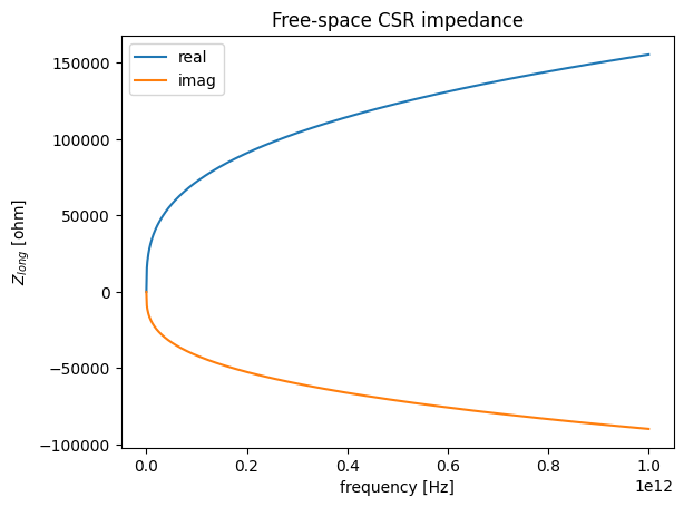
Impedance

The impedance is computed using Eq. (A10) of [2]:

\[Z_\parallel(\omega) = \frac{Z_0 L}{2\pi}\,\Gamma\!\left(\frac{2}{3}\right) \left(\frac{-i\omega}{3c R^2}\right)^{1/3}\]

where \(Z_0 = \mu_0 c\) is the impedance of free space, \(L\) is the length of the element, \(R\) is the bending radius, and \(\Gamma\) is the Euler gamma function.

Wake function

The free-space CSR wake function is singular at \(\tau = 0^-\). Two equivalent representations are implemented.

Direct wake function (Saldin et al. [3]):

\[W_\parallel(\tau) = -\frac{L}{\pi\varepsilon_0}\frac{\gamma^4}{R^2}\left[A + \frac{B}{C}\right], \quad \tau < 0\]

where \(A\), \(B\), \(C\) are functions of the normalised time \(\bar{s} = -\tau c\gamma^3/R\).

Antiderivative method (Murphy et al. [4]):

Because the direct wake function diverges as \(\tau \to 0^-\), a numerically more accurate approach convolves the antiderivative \(V(\tau) = \int_{-\infty}^{\tau} W_\parallel(\tau')\,d\tau'\) with the derivative of the bunch profile \(\lambda'(\tau)\):

\[W_p(\tau) = \int_{-\infty}^{\infty} \lambda'(\tau') \, V(\tau - \tau') \, d\tau'\]

This is the default method used in mbtrack2 for FreeSpaceCSR. The antiderivative is stored as the Wcsr component of the WakeField (type 'csr'), while the direct wake function is available via LongitudinalWakeFunction but is not added to the model by default.

Creating a FreeSpaceCSR object

The main parameters are:

• time: time array where the antiderivative wake function is evaluated, in [s].

• frequency: frequency array for the impedance, in [Hz].

• length: effective length contributing to CSR, in [m].

• radius: dipole bending radius \(R\), in [m].

• ring: the Synchrotron object (used for \(\gamma\)).

R = 5.36         # Dipole bending radius in [m].
L_csr = ring.L   # Effective CSR length = ring circumference in [m].

# Time grid for tracking: spans the bunch (20 sigma_0 on each side).
t = np.linspace(-20 * ring.sigma_0, 20 * ring.sigma_0, 10_001)

# Frequency grid for the impedance up to 1 THz.
frequency = np.linspace(0, 1e12, 1000)  # in [Hz]

csr_fs = FreeSpaceCSR(time=t, frequency=frequency, length=L_csr, radius=R, ring=ring)
print(csr_fs)

WakeField None with components:
 [np.str_('Wcsr'), np.str_('Zlong')]

The FreeSpaceCSR object has two components:

• Zlong: the longitudinal impedance.

• Wcsr: the antiderivative of the wake function (type 'csr'), used by WakePotential.

csr_fs.components

array(['Wcsr', 'Zlong'], dtype='<U5')

Plotting the impedance

%matplotlib inline
ax = csr_fs.Zlong.plot()
ax.set_title("Free-space CSR impedance")

Text(0.5, 1.0, 'Free-space CSR impedance')

Plotting the wake function and its antiderivative

The wake function shape is resolved in the normalised coordinate \(\mu = \frac{3\gamma^3}{2R}\,s\) (where \(s = c\tau\) is the longitudinal position). To visualise it, a dedicated fine spatial grid is used — independent of the bunch-spanning time grid used for tracking.

# Dedicated spatial grid for wake function shape visualisation (in meters).
s_wf = np.linspace(-1e-8, 1e-8, 10_001)
mu = 3 * ring.gamma**3 / (2 * R) * s_wf  # normalised coordinate

# Direct wake function (Saldin et al.) — call the method with this fine grid.
W_direct = csr_fs.LongitudinalWakeFunction(time=s_wf / c)

# Antiderivative (Murphy et al.) — also called directly on the fine grid.
V_antiderivative = csr_fs.LongitudinalWakeAntiderivative(time=s_wf / c)

fig, axes = plt.subplots(1, 2, figsize=(12, 4))

W_norm = np.nanmax(np.abs(W_direct[s_wf < 0]))
axes[0].plot(mu, W_direct / W_norm)
axes[0].set_xlim(-10, 2)
axes[0].set_ylim(-0.1, 0.5)
axes[0].axhline(0, color='gray', ls='-.', lw=0.8)
axes[0].axvline(-2.7, color='gray', ls='-.', lw=0.8)
axes[0].set_xlabel(r'Normalised time $\mu = \frac{3\gamma^3}{2R}\,s$')
axes[0].set_ylabel(r'$W_\parallel(\mu)$ (normalised)')
axes[0].set_title('Free-space CSR wake function (Saldin et al.)')

V_norm = np.nanmax(np.abs(V_antiderivative[s_wf < 0]))
axes[1].plot(mu, V_antiderivative / V_norm)
axes[1].set_xlim(-10, 2)
axes[1].axhline(0, color='gray', ls='-.', lw=0.8)
axes[1].axvline(-2.7, color='gray', ls='-.', lw=0.8)
axes[1].set_xlabel(r'Normalised time $\mu = \frac{3\gamma^3}{2R}\,s$')
axes[1].set_ylabel(r'$V(\mu)$ (normalised)')
axes[1].set_title('Antiderivative of CSR wake function (Murphy et al.)')

plt.tight_layout()

print(f"Wake function zero crossing at mu = -2.7, i.e. s = {1.8*R/ring.gamma**3*1e12:.2e} pm")

Wake function zero crossing at mu = -2.7, i.e. s = 6.19e+01 pm

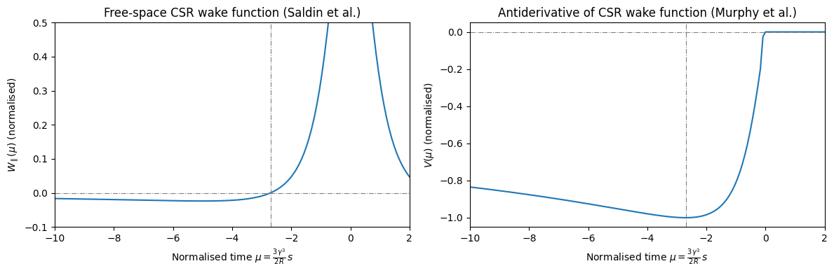
The wake function changes sign at \(\mu \approx -2.7\) and diverges as \(\mu \to 0^-\). The antiderivative \(V(\mu)\) is smooth everywhere and reaches zero at \(\mu = 0\), making it much better suited for numerical convolution.

Parallel-plates CSR: ParallelPlatesCSR

Physical model

When the beam pipe is modelled as two perfectly conducting parallel plates separated by a full-gap distance \(h\), the CSR field is shielded at long wavelengths. This shielding suppresses the CSR emission below the threshold frequency:

\[f_{\rm th} = \frac{3c}{2\pi}\left(\frac{R}{h^3}\right)^{1/2}\]

Above threshold, the radiation spectrum is essentially the same as free space. Below threshold, the CSR power is strongly suppressed.

The ParallelPlatesCSR class provides:

• Impedance (Zlong): Eq. (A1) of [2] (Agoh-Yokoya sum formula), which includes both free-space and shielding contributions.

• Shielding wake (Wlong): Eqs. (5.21-5.22) of [4] (Murphy et al. G2 function), which contains only the shielding correction.

• Free-space wake (Wcsr): antiderivative of the free-space wake, automatically included by calling FreeSpaceCSR internally. This makes the time-domain model consistent with the frequency-domain impedance.

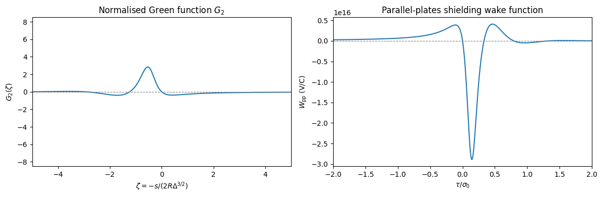
Approximation used for the wake function

The parallel-plates wake function is computed via the normalised Green’s function \(G_2(\zeta)\), where \(\zeta = -s / (2R\Delta^{3/2})\) and \(\Delta = h/(2R)\):

\[G_2(\zeta) = \sum_{k=1}^{k_{\rm max}} \frac{2(-1)^{k+1}}{k^2} \frac{4Y_k^4(3 - Y_k^4)}{(1 + Y_k^4)^3}\]

where \(Y_k(\zeta)\) is the real positive root of a characteristic polynomial (Eq. 5.18 of [4]). The sum is truncated at k_max terms. The amplitude coefficient is:

\[W_{\rm pp}(\tau) = -\frac{4L}{8\pi\varepsilon_0\, h^2}\, G_2\!\left(-c\tau\right)\]

Creating a ParallelPlatesCSR object

In addition to the parameters of FreeSpaceCSR, ParallelPlatesCSR requires:

• distance: full-gap vertical separation between the plates \(h\), in [m].

• k_max (optional): number of terms in the image-charge sum (default 100).

Note: the impedance computation uses mpmath and can be slow for large frequency arrays. The wake function also uses a 2D root-finding loop and can take several seconds for a fine time grid.

h_gap = 2*12.5e-3  # Full gap distance between the plates in [m].

# Time grid: use the same bunch-spanning grid as for FreeSpaceCSR.
# A coarser step is used here to keep computation time reasonable.
t_pp = np.arange(-5e-11, 5e-11, 1e-13)  # in [s]

csr_pp = ParallelPlatesCSR(
    time=t_pp,
    frequency=np.linspace(1, 2e12, 500),  # up to 1 THz
    length=L_csr,
    radius=R,
    distance=h_gap,
    ring=ring,
    k_max=25,
)
print(csr_pp)

WakeField None with components:
 [np.str_('Wcsr'), np.str_('Wlong'), np.str_('Zlong')]

The ParallelPlatesCSR object has three components:

• Zlong: the full longitudinal impedance (free space + shielding).

• Wlong: the shielding-only wake function (type 'long', standard convolution).

• Wcsr: the free-space CSR antiderivative (type 'csr', derivative convolution), automatically included for a complete time-domain model.

csr_pp.components

array(['Wcsr', 'Wlong', 'Zlong'], dtype='<U5')

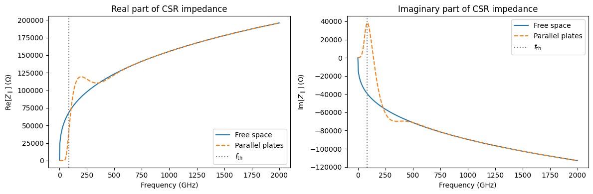
Shielding threshold

print(f"Shielding threshold: {csr_pp.threshold/1e9:.2f} GHz")
print(f"Delta = h/(2R) = {h_gap/(2*R):.4f}")

Shielding threshold: 83.84 GHz
Delta = h/(2R) = 0.0023

Plotting the impedance

The real part of the parallel-plates impedance is suppressed below the shielding threshold compared to the free-space model.

# Recompute free-space impedance on the same frequency grid for comparison.
freq_compare = np.linspace(1, 2e12, 500)  # up to 1 THz
Z_fs = csr_fs.LongitudinalImpedance(freq_compare)
Z_pp = csr_pp.Zlong.data

fig, axes = plt.subplots(1, 2, figsize=(12, 4))

axes[0].plot(freq_compare / 1e9, Z_fs.real, label='Free space', lw=1.5)
axes[0].plot(freq_compare / 1e9, Z_pp.real, label='Parallel plates', lw=1.5, ls='--')
axes[0].axvline(csr_pp.threshold / 1e9, color='gray', ls=':', label=r'$f_{\rm th}$')
axes[0].set_xlabel('Frequency (GHz)')
axes[0].set_ylabel(r'Re[$Z_\parallel$] ($\Omega$)')
axes[0].set_title('Real part of CSR impedance')
axes[0].legend()

axes[1].plot(freq_compare / 1e9, Z_fs.imag, label='Free space', lw=1.5)
axes[1].plot(freq_compare / 1e9, Z_pp.imag, label='Parallel plates', lw=1.5, ls='--')
axes[1].axvline(csr_pp.threshold / 1e9, color='gray', ls=':', label=r'$f_{\rm th}$')
axes[1].set_xlabel('Frequency (GHz)')
axes[1].set_ylabel(r'Im[$Z_\parallel$] ($\Omega$)')
axes[1].set_title('Imaginary part of CSR impedance')
axes[1].legend()

plt.tight_layout()

Plotting the \(G_2\) function and the parallel-plates wake function

The normalised Green’s function \(G_2(\zeta)\) characterises the shape of the shielding correction. It oscillates with decreasing amplitude around zero for \(|\zeta| \gg 1\).

delta = h_gap / (2 * R)
s_pp = t_pp * c
zeta = -s_pp / (2 * R * delta**(3/2))  # normalised coordinate

G2 = csr_pp._G2(s_pp)

fig, axes = plt.subplots(1, 2, figsize=(12, 4))

axes[0].plot(zeta, G2)
axes[0].axhline(0, color='gray', ls='--', lw=0.8)
axes[0].set_xlim(-5, 5)
axes[0].set_ylim(-8.5, 8.5)
axes[0].set_xlabel(r'$\zeta = -s/(2R\Delta^{3/2})$')
axes[0].set_ylabel(r'$G_2(\zeta)$')
axes[0].set_title('Normalised Green function $G_2$')

axes[1].plot(t_pp / ring.sigma_0, csr_pp.Wlong.data.real)
axes[1].axhline(0, color='gray', ls='--', lw=0.8)
axes[1].set_xlim(-2, 2)
axes[1].set_xlabel(r'$\tau / \sigma_0$')
axes[1].set_ylabel(r'$W_{\rm pp}$ (V/C)')
axes[1].set_title('Parallel-plates shielding wake function')

plt.tight_layout()

Using CSR wakefields in tracking

Both FreeSpaceCSR and ParallelPlatesCSR are used with the WakePotential class for single-bunch tracking. The WakePotential computes the wake potential by convolving the wake function with the bunch charge profile, then applies the resulting voltage kick to each macroparticle.

Key difference: Wcsr vs Wlong

The two component types use different convolution algorithms:

Component	wake_type	Algorithm
Wcsr	"Wcsr"	Convolves antiderivative \(V(\tau)\) with \(\lambda'(\tau)\) (derivative of profile)
Wlong	"Wlong"	Standard convolution of \(W_{\rm pp}(\tau)\) with \(\lambda(\tau)\)

ParallelPlatesCSR has both components, so WakePotential will apply both convolutions each turn. The correct algorithm is triggered automatically by WakePotential based on the component type.

Fine time grid for tracking

Both CSR models are rebuilt on a single common time grid spanning ±30 σ₀ with step σ₀/500. This grid is wide enough to cover the full bunch and fine enough to resolve the oscillatory shielding wake of ParallelPlatesCSR.

dtau_track = ring.sigma_0 / 500
t_track = np.arange(-30 * ring.sigma_0, 30 * ring.sigma_0, dtau_track)

csr_fs = FreeSpaceCSR(time=t_track, frequency=frequency, length=L_csr, radius=R, ring=ring)
csr_pp = ParallelPlatesCSR(
    time=t_track,
    frequency=np.linspace(1, 2e12, 500),
    length=L_csr,
    radius=R,
    distance=h_gap,
    ring=ring,
    k_max=100,
)
print(f"Time grid: {len(t_track)} points, step = {dtau_track * 1e12:.2f} ps, span = ±{20 * ring.sigma_0 * 1e12:.0f} ps")

Time grid: 30000 points, step = 0.03 ps, span = ±300 ps

Wake potential for FreeSpaceCSR

We first initialise a bunch at equilibrium, then compute the wake potential from a single call to wp_fs.track from the actual simulated bunch profile. We then compare it with the perfect-Gaussian bunch profile from plot_gaussian_wake.

bunch_fs = Bunch(ring, mp_number=5_000_000, current=10e-3)
bunch_fs.init_gaussian()
wp_fs = WakePotential(ring, csr_fs, n_bin=200)
wp_fs.track(bunch_fs)

The WakePotential frequency cutoff (from WakeFunction time array definition and from Bunch binning) can be checked by using:

print(f"Max frequency taken into account in tracking: {wp_fs.wakepotential_max_frequency*1e-9:.2f} GHz")

Max frequency taken into account in tracking: 614.23 GHz

fig, axes = plt.subplots(2, 1, figsize=(10, 8))

wp_fs.plot_gaussian_wake(ring.sigma_0, wake_type="Wcsr", ax=axes[0])
axes[0].set_title("Gaussian wake (Wcsr)")

wp_fs.plot_last_wake("Wcsr", ax=axes[1])
axes[1].set_title("Tracked wake (Wcsr)")

plt.tight_layout()

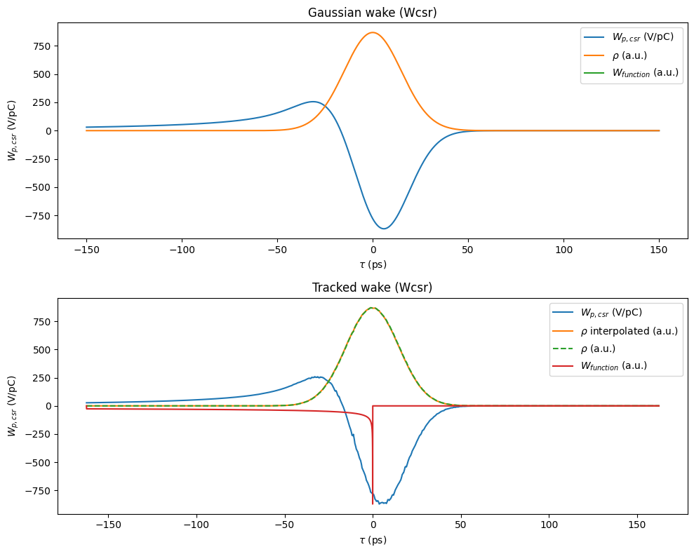
The typical free space CSR wake potential shows a net energy loss at the bunch tail and an energy gain at the head.

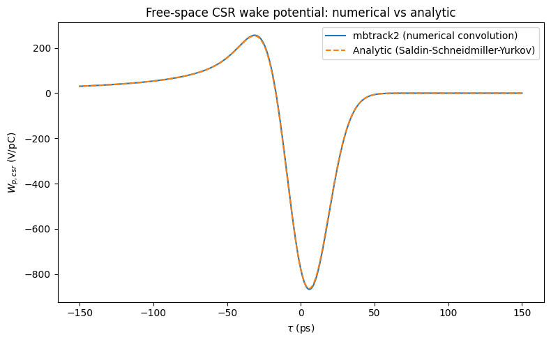
Comparison with the analytic Gaussian solution

For a perfectly Gaussian bunch in the free-space, steady-state CSR regime, the wake potential has a closed-form expression in terms of the parabolic cylinder function (Saldin-Schneidmiller-Yurkov):

\[W_p(s) = -\frac{1}{4\pi\varepsilon_0}\,\sqrt{\frac{2}{\pi}}\,\frac{\Gamma(2/3)}{(3R^2\sigma^4)^{1/3}}\,\exp\!\left(-\frac{s^2}{4\sigma^2}\right)\,D_{1/3}\!\left(-\frac{s}{\sigma}\right)\]

where \(s = c\tau\), \(R\) is the bending radius, \(\sigma\) is the RMS bunch length in [m], and \(D_\nu\) is the parabolic cylinder function. This expression gives the wake potential per unit dipole length, so it must be multiplied by ring.L (the effective CSR length used in FreeSpaceCSR) to be compared with the mbtrack2 numerical result.

from scipy.special import pbdv, gamma
from scipy.constants import epsilon_0

def get_gaussian_csr_wakepotential(s, rho, sigma):
    coeff = -1/(4*pi*epsilon_0) * np.sqrt(2/pi) / (3 * rho**2 * sigma**4)**(1/3)
    return coeff * gamma(2/3) * np.exp(-.25*(s/sigma)**2) * pbdv(1/3, -s/sigma)[0]

t_analytic = np.linspace(-10 * ring.sigma_0, 10 * ring.sigma_0, 2902)
Wp_analytic = get_gaussian_csr_wakepotential(c * t_analytic, R, ring.sigma_0 * c) * ring.L

tau0_num, _, Wp_num, _, _ = wp_fs.get_gaussian_wakepotential(ring.sigma_0, "Wcsr")

fig, ax = plt.subplots(figsize=(8, 5))
ax.plot(tau0_num * 1e12, Wp_num * 1e-12, label="mbtrack2 (numerical convolution)")
ax.plot(-t_analytic * 1e12, Wp_analytic * 1e-12, ls='--', label="Analytic (Saldin-Schneidmiller-Yurkov)")
ax.set_xlabel(r"$\tau$ (ps)")
ax.set_ylabel(r"$W_{p,csr}$ (V/pC)")
ax.set_title("Free-space CSR wake potential: numerical vs analytic")
ax.legend()
plt.tight_layout()

Wake potential for ParallelPlatesCSR

Fully shielded regime

Since ParallelPlatesCSR contains both Wlong and Wcsr, we can retrieve and plot each contribution separately.

Top row: Gaussian predictions. Bottom row: wake potentials from plot_last_wake after a single wp_pp.track call.

bunch_pp = Bunch(ring, mp_number=5_000_000, current=10e-3)
bunch_pp.init_gaussian()
wp_pp = WakePotential(ring, csr_pp, n_bin=128)
wp_pp.track(bunch_pp)

fig, axes = plt.subplots(2, 3, figsize=(18, 8))

wp_pp.plot_gaussian_wake(ring.sigma_0, wake_type="Wlong", plot_wake_function=False, ax=axes[0, 0])
axes[0, 0].set_title("Gaussian: shielding (Wlong)")

wp_pp.plot_gaussian_wake(ring.sigma_0, wake_type="Wcsr", plot_wake_function=False, ax=axes[0, 1])
axes[0, 1].set_title("Gaussian: free-space (Wcsr)")

wp_pp.plot_gaussian_wake(ring.sigma_0, wake_type="Wcsr", plot_full_csr_wake=True, plot_wake_function=False, ax=axes[0, 2])
axes[0, 2].set_title("Gaussian: total (Wcsr + Wlong)")

wp_pp.plot_last_wake("Wlong", plot_wake_function=False, ax=axes[1, 0])
axes[1, 0].set_title("Tracked: shielding (Wlong)")

wp_pp.plot_last_wake("Wcsr", plot_wake_function=False, ax=axes[1, 1])
axes[1, 1].set_title("Tracked: free-space (Wcsr)")

wp_pp.plot_last_wake("Wcsr", plot_full_csr_wake=True, plot_wake_function=False, ax=axes[1, 2])
axes[1, 2].set_title("Tracked: total (Wcsr + Wlong)")

plt.tight_layout()

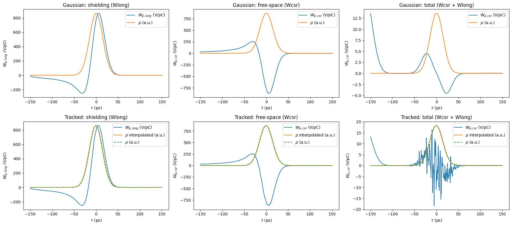
As it is visible in tracking total wake for Wcsr + Wlong, the ParallelPlateCSR can be quite sensitive to noise when in the shielded regime. This is due to:

• The Wcsr dependancy on the derivative of bunch profile.

• The near perfect cancellation of Wcsr and Wlong.

In that case, a convergence study needs to be done to check the influence of numerical noise on beam dynamics results.

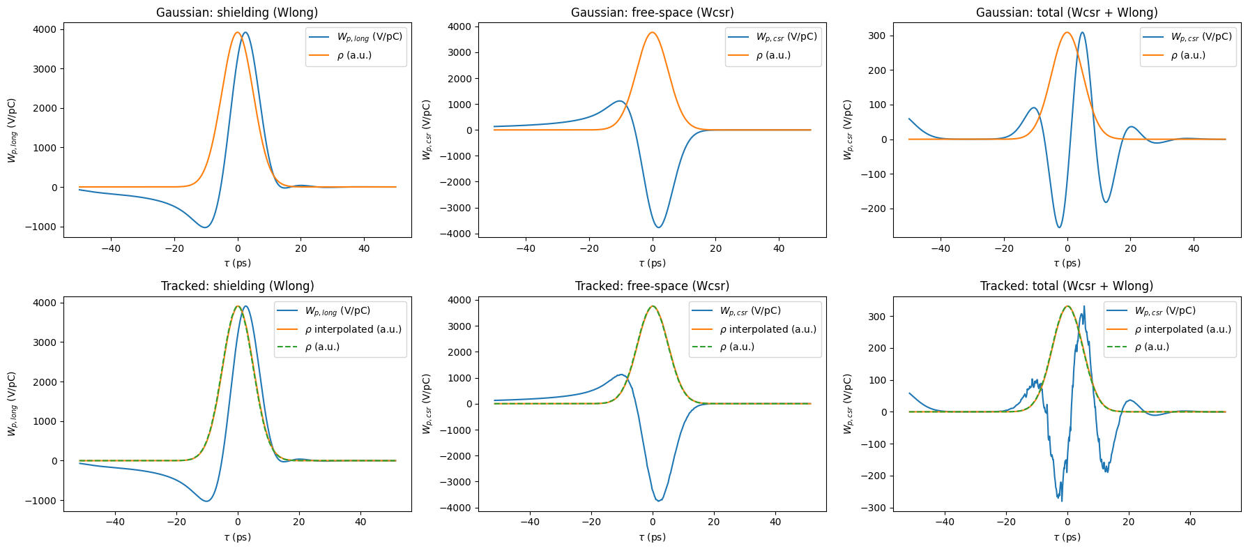
Partialy shielded regime

If the bunch length is reduced, the beam frequency reached is increased and the effect of numerical noise is reduced.

ring.sigma_0 = 5e-12

bunch_pp = Bunch(ring, mp_number=5_000_000, current=10e-3)
bunch_pp.init_gaussian()
wp_pp = WakePotential(ring, csr_pp, n_bin=128)
wp_pp.track(bunch_pp)

fig, axes = plt.subplots(2, 3, figsize=(18, 8))

wp_pp.plot_gaussian_wake(ring.sigma_0, wake_type="Wlong", plot_wake_function=False, ax=axes[0, 0])
axes[0, 0].set_title("Gaussian: shielding (Wlong)")

wp_pp.plot_gaussian_wake(ring.sigma_0, wake_type="Wcsr", plot_wake_function=False, ax=axes[0, 1])
axes[0, 1].set_title("Gaussian: free-space (Wcsr)")

wp_pp.plot_gaussian_wake(ring.sigma_0, wake_type="Wcsr", plot_full_csr_wake=True, plot_wake_function=False, ax=axes[0, 2])
axes[0, 2].set_title("Gaussian: total (Wcsr + Wlong)")

wp_pp.plot_last_wake("Wlong", plot_wake_function=False, ax=axes[1, 0])
axes[1, 0].set_title("Tracked: shielding (Wlong)")

wp_pp.plot_last_wake("Wcsr", plot_wake_function=False, ax=axes[1, 1])
axes[1, 1].set_title("Tracked: free-space (Wcsr)")

wp_pp.plot_last_wake("Wcsr", plot_full_csr_wake=True, plot_wake_function=False, ax=axes[1, 2])
axes[1, 2].set_title("Tracked: total (Wcsr + Wlong)")

plt.tight_layout()

Summary

	FreeSpaceCSR	ParallelPlatesCSR
Model	Steady-state, no boundaries	Steady-state + perfectly conducting plates
Impedance formula	Agoh-Yokoya Eq. (A10)	Agoh-Yokoya Eq. (A1), sum over image charges
Zlong	Yes	Yes (free space + shielding)
Wlong	No	Yes (shielding correction, \(G_2\) function)
Wcsr	Yes (antiderivative \(V(\tau)\))	Yes (automatically included via FreeSpaceCSR)
Convolution for Wcsr	\(V(\tau) \star \lambda'(\tau)\)	\(V(\tau) \star \lambda'(\tau)\)
Convolution for Wlong	N/A	\(W_{\rm pp}(\tau) \star \lambda(\tau)\)
Shielding	None	Suppressed below \(f_{\rm th}\)
Complete time-domain model	Yes	Yes